In Part 3, we have reviewed models in the R-CNN family. All of them are region-based object detection algorithms. They can achieve high accuracy but could be too slow for certain applications such as autonomous driving. In Part 4, we only focus on fast object detection models, including SSD, RetinaNet, and models in the YOLO family.

Links to all the posts in the series: [Part 1] [Part 2] [Part 3] [Part 4].

Two-stage vs One-stage Detectors

Models in the R-CNN family are all region-based. The detection happens in two stages: (1) First, the model proposes a set of regions of interests by select search or regional proposal network. The proposed regions are sparse as the potential bounding box candidates can be infinite. (2) Then a classifier only processes the region candidates.

The other different approach skips the region proposal stage and runs detection directly over a dense sampling of possible locations. This is how a one-stage object detection algorithm works. This is faster and simpler, but might potentially drag down the performance a bit.

All the models introduced in this post are one-stage detectors.

YOLO: You Only Look Once

The YOLO model (“You Only Look Once”; Redmon et al., 2016) is the very first attempt at building a fast real-time object detector. Because YOLO does not undergo the region proposal step and only predicts over a limited number of bounding boxes, it is able to do inference super fast.

Workflow

1. Pre-train a CNN network on image classification task.

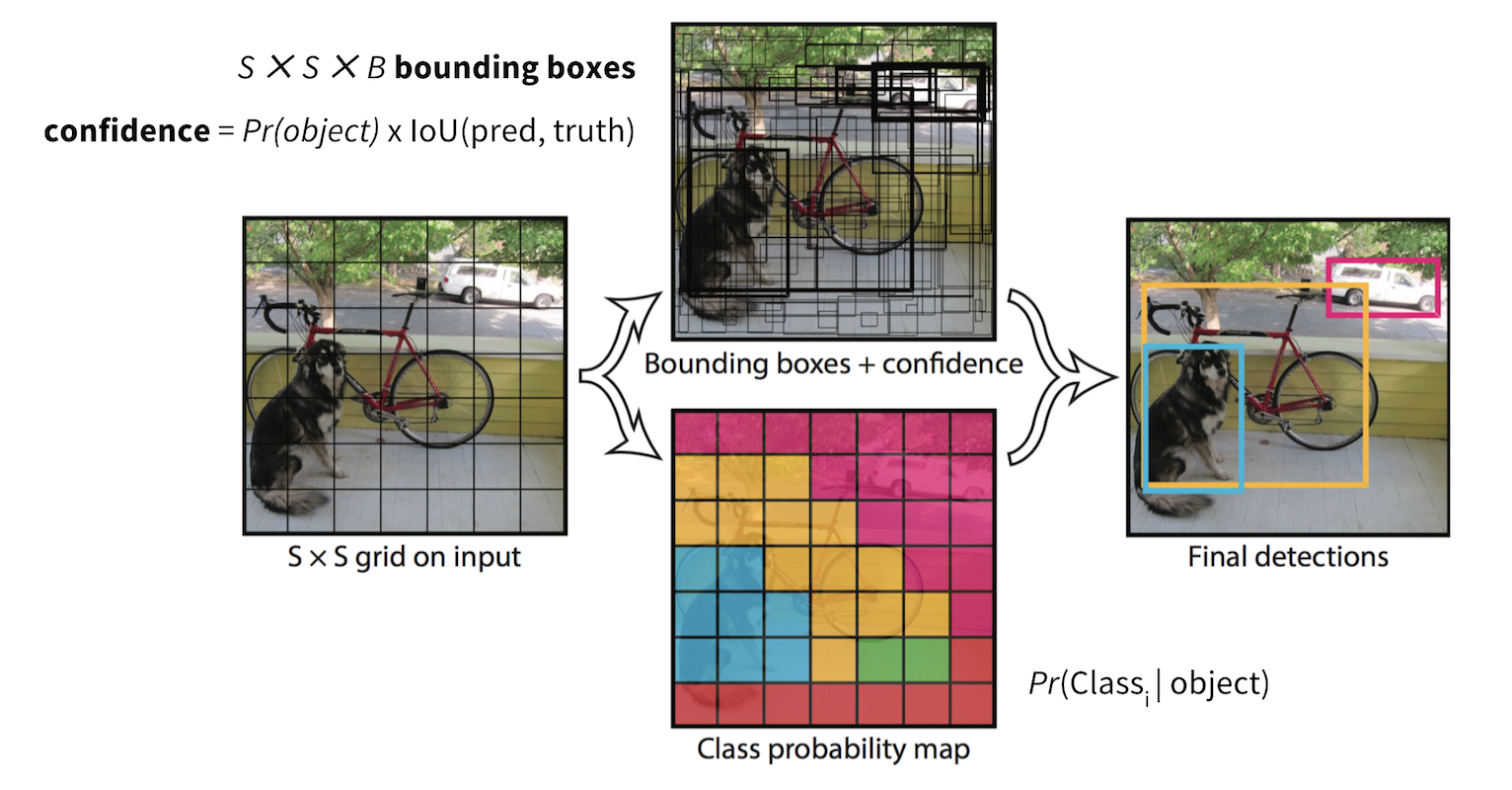
2. Split an image into $S \times S$ cells. If an object’s center falls into a cell, that cell is “responsible” for detecting the existence of that object. Each cell predicts (a) the location of $B$ bounding boxes, (b) a confidence score, and (c) a probability of object class conditioned on the existence of an object in the bounding box.

   • The coordinates of bounding box are defined by a tuple of 4 values, (center x-coord, center y-coord, width, height) — $(x, y, w, h)$, where $x$ and $y$ are set to be offset of a cell location. Moreover, $x$, $y$, $w$ and $h$ are normalized by the image width and height, and thus all between (0, 1].
   • A confidence score indicates the likelihood that the cell contains an object: Pr(containing an object) x IoU(pred, truth); where Pr = probability and IoU = interaction under union.
   • If the cell contains an object, it predicts a probability of this object belonging to every class $C_i, i=1, \dots, K$: Pr(the object belongs to the class C_i | containing an object). At this stage, the model only predicts one set of class probabilities per cell, regardless of the number of bounding boxes, $B$.
   • In total, one image contains $S \times S \times B$ bounding boxes, each box corresponding to 4 location predictions, 1 confidence score, and K conditional probabilities for object classification. The total prediction values for one image is $S \times S \times (5B + K)$, which is the tensor shape of the final conv layer of the model.

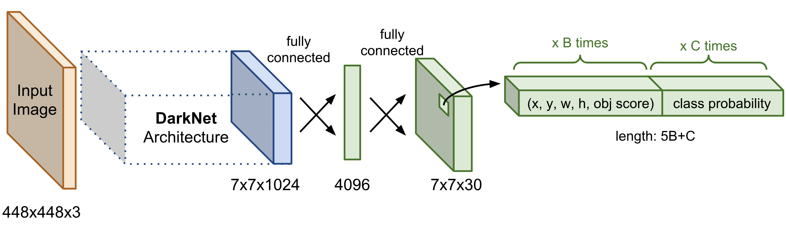
3. The final layer of the pre-trained CNN is modified to output a prediction tensor of size $S \times S \times (5B + K)$.

Network Architecture

The base model is similar to GoogLeNet with inception module replaced by 1x1 and 3x3 conv layers. The final prediction of shape $S \times S \times (5B + K)$ is produced by two fully connected layers over the whole conv feature map.

Loss Function

The loss consists of two parts, the localization loss for bounding box offset prediction and the classification loss for conditional class probabilities. Both parts are computed as the sum of squared errors. Two scale parameters are used to control how much we want to increase the loss from bounding box coordinate predictions ($\lambda_\text{coord}$) and how much we want to decrease the loss of confidence score predictions for boxes without objects ($\lambda_\text{noobj}$). Down-weighting the loss contributed by background boxes is important as most of the bounding boxes involve no instance. In the paper, the model sets $\lambda_\text{coord} = 5$ and $\lambda_\text{noobj} = 0.5$.

NOTE: In the original YOLO paper, the loss function uses $C_i$ instead of $C_{ij}$ as confidence score. I made the correction based on my own understanding, since every bounding box should have its own confidence score. Please kindly let me if you do not agree. Many thanks.

where,

• $\mathbb{1}_i^\text{obj}$: An indicator function of whether the cell i contains an object.
• $\mathbb{1}_{ij}^\text{obj}$: It indicates whether the j-th bounding box of the cell i is “responsible” for the object prediction (see Fig. 3).
• $C_{ij}$: The confidence score of cell i, Pr(containing an object) * IoU(pred, truth).
• $\hat{C}_{ij}$: The predicted confidence score.
• $\mathcal{C}$: The set of all classes.
• $p_i(c)$: The conditional probability of whether cell i contains an object of class $c \in \mathcal{C}$.
• $\hat{p}_i(c)$: The predicted conditional class probability.

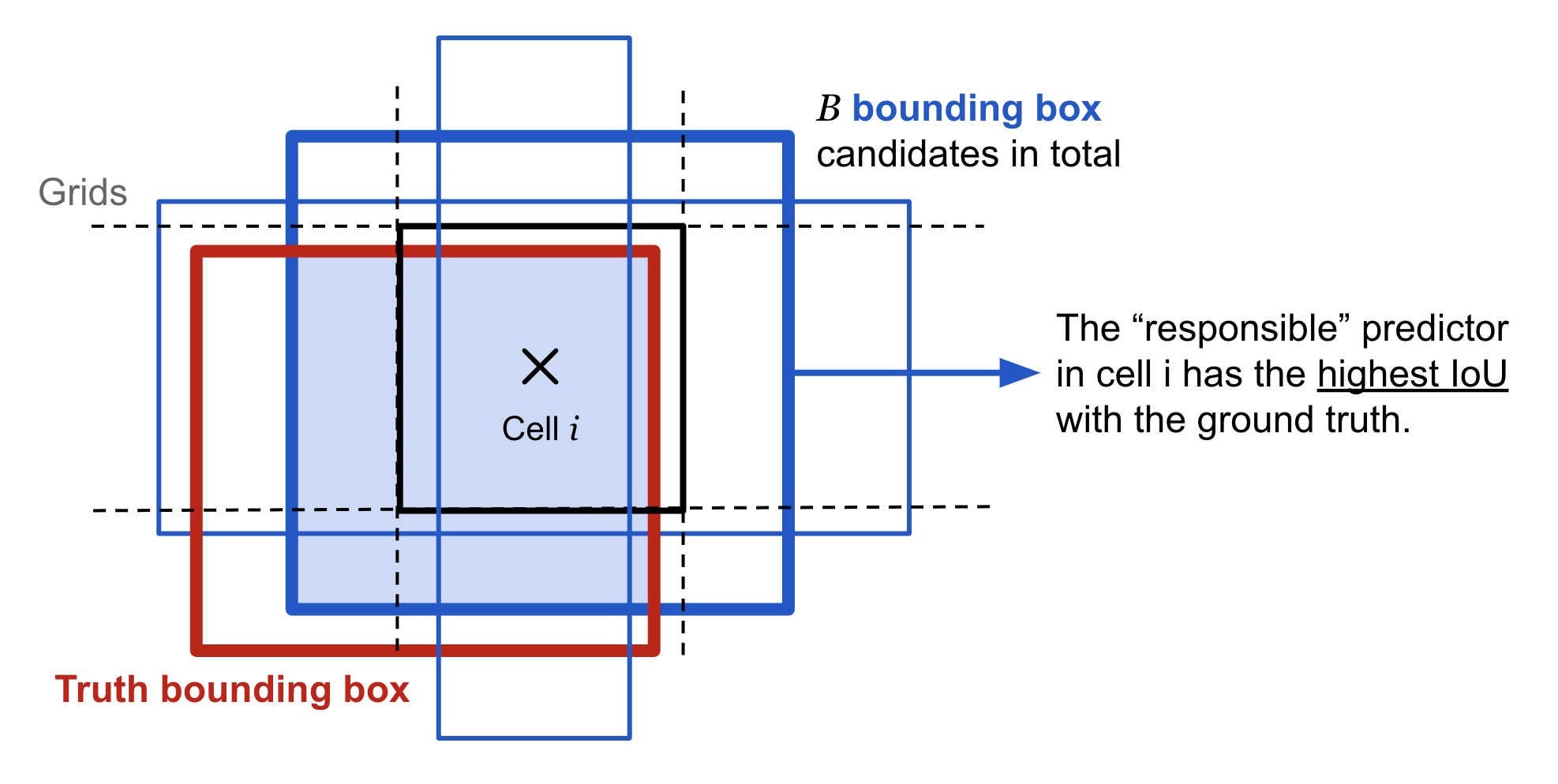
The loss function only penalizes classification error if an object is present in that grid cell, $\mathbb{1}_i^\text{obj} = 1$. It also only penalizes bounding box coordinate error if that predictor is “responsible” for the ground truth box, $\mathbb{1}_{ij}^\text{obj} = 1$.

As a one-stage object detector, YOLO is super fast, but it is not good at recognizing irregularly shaped objects or a group of small objects due to a limited number of bounding box candidates.

SSD: Single Shot MultiBox Detector

The Single Shot Detector (SSD; Liu et al, 2016) is one of the first attempts at using convolutional neural network’s pyramidal feature hierarchy for efficient detection of objects of various sizes.

Image Pyramid

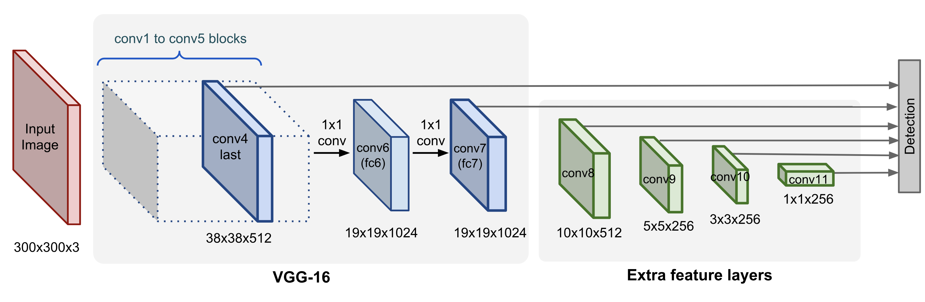
SSD uses the VGG-16 model pre-trained on ImageNet as its base model for extracting useful image features. On top of VGG16, SSD adds several conv feature layers of decreasing sizes. They can be seen as a pyramid representation of images at different scales. Intuitively large fine-grained feature maps at earlier levels are good at capturing small objects and small coarse-grained feature maps can detect large objects well. In SSD, the detection happens in every pyramidal layer, targeting at objects of various sizes.

Workflow

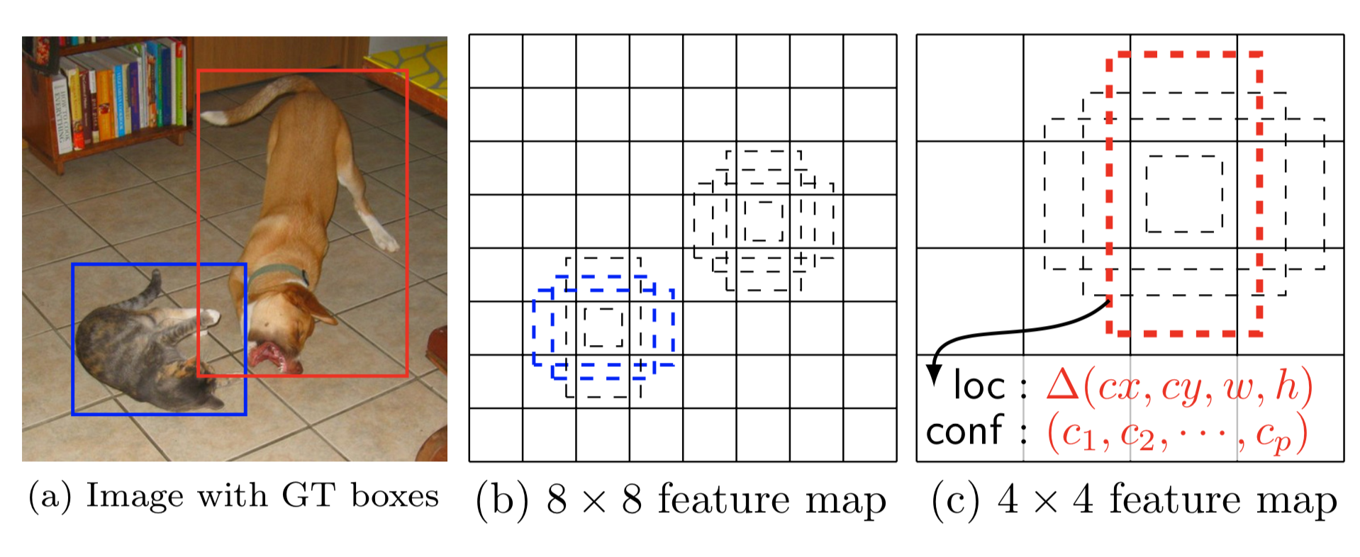
Unlike YOLO, SSD does not split the image into grids of arbitrary size but predicts offset of predefined anchor boxes (this is called “default boxes” in the paper) for every location of the feature map. Each box has a fixed size and position relative to its corresponding cell. All the anchor boxes tile the whole feature map in a convolutional manner.

Feature maps at different levels have different receptive field sizes. The anchor boxes on different levels are rescaled so that one feature map is only responsible for objects at one particular scale. For example, in Fig. 5 the dog can only be detected in the 4x4 feature map (higher level) while the cat is just captured by the 8x8 feature map (lower level).

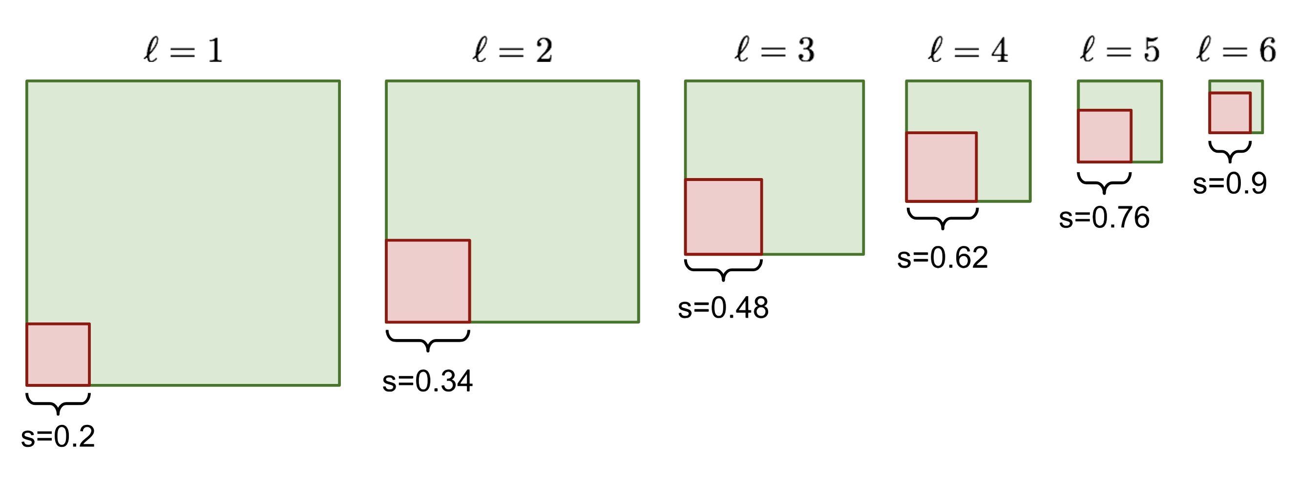
The width, height and the center location of an anchor box are all normalized to be (0, 1). At a location $(i, j)$ of the $\ell$-th feature layer of size $m \times n$, $i=1,\dots,n, j=1,\dots,m$, we have a unique linear scale proportional to the layer level and 5 different box aspect ratios (width-to-height ratios), in addition to a special scale (why we need this? the paper didn’t explain. maybe just a heuristic trick) when the aspect ratio is 1. This gives us 6 anchor boxes in total per feature cell.

At every location, the model outputs 4 offsets and $c$ class probabilities by applying a $3 \times 3 \times p$ conv filter (where $p$ is the number of channels in the feature map) for every one of $k$ anchor boxes. Therefore, given a feature map of size $m \times n$, we need $kmn(c+4)$ prediction filters.

Loss Function

Same as YOLO, the loss function is the sum of a localization loss and a classification loss.

$\mathcal{L} = \frac{1}{N}(\mathcal{L}_\text{cls} + \alpha \mathcal{L}_\text{loc})$

where $N$ is the number of matched bounding boxes and $\alpha$ balances the weights between two losses, picked by cross validation.

The localization loss is a smooth L1 loss between the predicted bounding box correction and the true values. The coordinate correction transformation is same as what R-CNN does in bounding box regression.

where $\mathbb{1}_{ij}^\text{match}$ indicates whether the $i$-th bounding box with coordinates $(p^i_x, p^i_y, p^i_w, p^i_h)$ is matched to the $j$-th ground truth box with coordinates $(g^j_x, g^j_y, g^j_w, g^j_h)$ for any object. $d^i_m, m\in\{x, y, w, h\}$ are the predicted correction terms. See this for how the transformation works.

The classification loss is a softmax loss over multiple classes (softmax_cross_entropy_with_logits in tensorflow):

where $\mathbb{1}_{ij}^k$ indicates whether the $i$-th bounding box and the $j$-th ground truth box are matched for an object in class $k$. $\text{pos}$ is the set of matched bounding boxes ($N$ items in total) and $\text{neg}$ is the set of negative examples. SSD uses hard negative mining to select easily misclassified negative examples to construct this $\text{neg}$ set: Once all the anchor boxes are sorted by objectiveness confidence score, the model picks the top candidates for training so that neg:pos is at most 3:1.

YOLOv2 / YOLO9000

YOLOv2 (Redmon & Farhadi, 2017) is an enhanced version of YOLO. YOLO9000 is built on top of YOLOv2 but trained with joint dataset combining the COCO detection dataset and the top 9000 classes from ImageNet.

YOLOv2 Improvement

A variety of modifications are applied to make YOLO prediction more accurate and faster, including:

1. BatchNorm helps: Add batch norm on all the convolutional layers, leading to significant improvement over convergence.

2. Image resolution matters: Fine-tuning the base model with high resolution images improves the detection performance.

3. Convolutional anchor box detection: Rather than predicts the bounding box position with fully-connected layers over the whole feature map, YOLOv2 uses convolutional layers to predict locations of anchor boxes, like in faster R-CNN. The prediction of spatial locations and class probabilities are decoupled. Overall, the change leads to a slight decrease in mAP, but an increase in recall.

4. K-mean clustering of box dimensions: Different from faster R-CNN that uses hand-picked sizes of anchor boxes, YOLOv2 runs k-mean clustering on the training data to find good priors on anchor box dimensions. The distance metric is designed to rely on IoU scores:

where $x$ is a ground truth box candidate and $c_i$ is one of the centroids. The best number of centroids (anchor boxes) $k$ can be chosen by the elbow method.

The anchor boxes generated by clustering provide better average IoU conditioned on a fixed number of boxes.

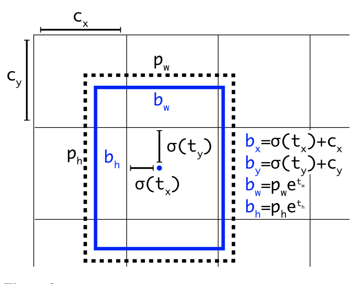
5. Direct location prediction: YOLOv2 formulates the bounding box prediction in a way that it would not diverge from the center location too much. If the box location prediction can place the box in any part of the image, like in regional proposal network, the model training could become unstable.

Given the anchor box of size $(p_w, p_h)$ at the grid cell with its top left corner at $(c_x, c_y)$, the model predicts the offset and the scale, $(t_x, t_y, t_w, t_h)$ and the corresponding predicted bounding box $b$ has center $(b_x, b_y)$ and size $(b_w, b_h)$. The confidence score is the sigmoid ($\sigma$) of another output $t_o$.

6. Add fine-grained features: YOLOv2 adds a passthrough layer to bring fine-grained features from an earlier layer to the last output layer. The mechanism of this passthrough layer is similar to identity mappings in ResNet to extract higher-dimensional features from previous layers. This leads to 1% performance increase.

7. Multi-scale training: In order to train the model to be robust to input images of different sizes, a new size of input dimension is randomly sampled every 10 batches. Since conv layers of YOLOv2 downsample the input dimension by a factor of 32, the newly sampled size is a multiple of 32.

8. Light-weighted base model: To make prediction even faster, YOLOv2 adopts a light-weighted base model, DarkNet-19, which has 19 conv layers and 5 max-pooling layers. The key point is to insert avg poolings and 1x1 conv filters between 3x3 conv layers.

YOLO9000: Rich Dataset Training

Because drawing bounding boxes on images for object detection is much more expensive than tagging images for classification, the paper proposed a way to combine small object detection dataset with large ImageNet so that the model can be exposed to a much larger number of object categories. The name of YOLO9000 comes from the top 9000 classes in ImageNet. During joint training, if an input image comes from the classification dataset, it only backpropagates the classification loss.

The detection dataset has much fewer and more general labels and, moreover, labels cross multiple datasets are often not mutually exclusive. For example, ImageNet has a label “Persian cat” while in COCO the same image would be labeled as “cat”. Without mutual exclusiveness, it does not make sense to apply softmax over all the classes.

In order to efficiently merge ImageNet labels (1000 classes, fine-grained) with COCO/PASCAL (< 100 classes, coarse-grained), YOLO9000 built a hierarchical tree structure with reference to WordNet so that general labels are closer to the root and the fine-grained class labels are leaves. In this way, “cat” is the parent node of “Persian cat”.

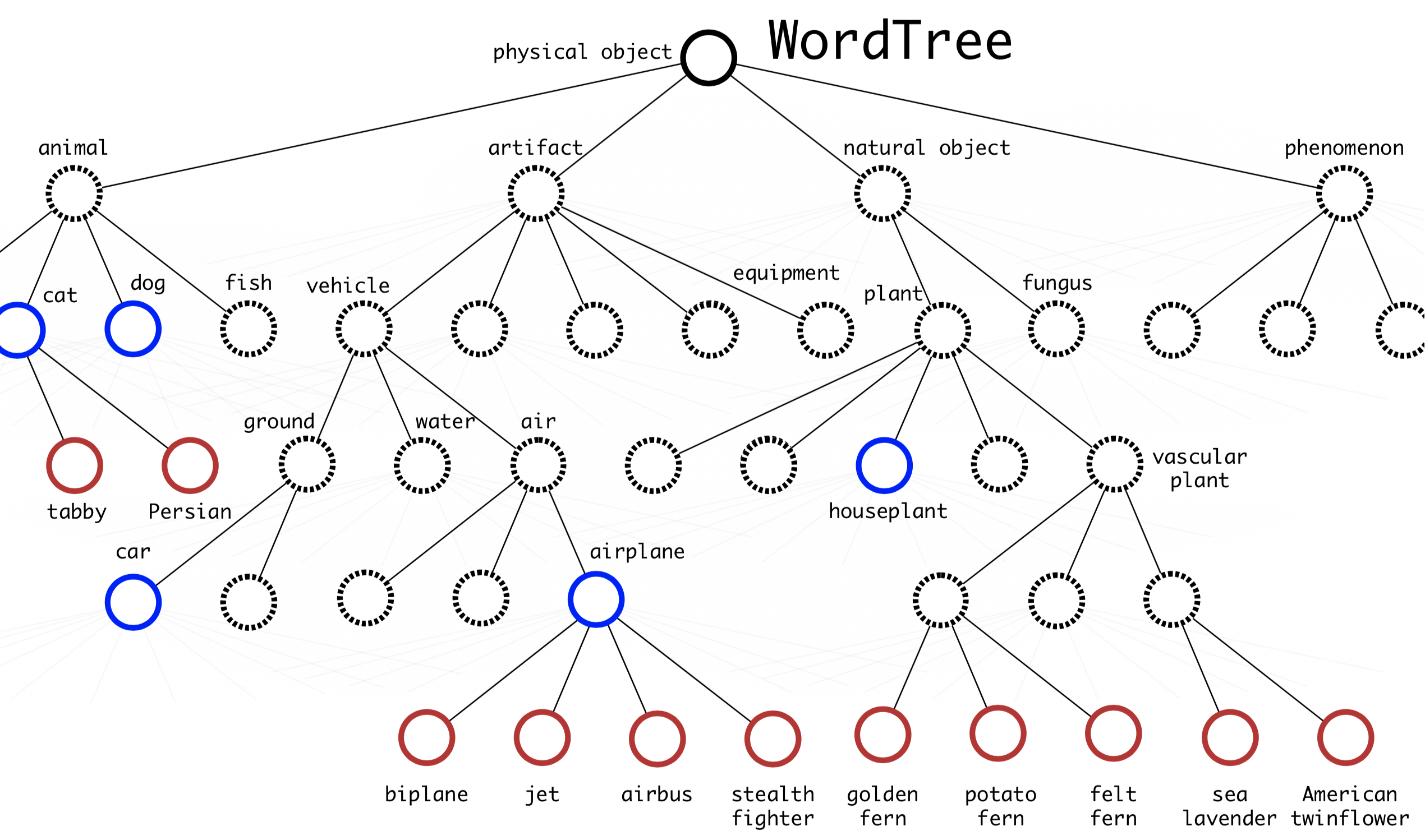
To predict the probability of a class node, we can follow the path from the node to the root:

Pr("persian cat" | contain a "physical object") 
= Pr("persian cat" | "cat") 
  Pr("cat" | "animal") 
  Pr("animal" | "physical object") 
  Pr(contain a "physical object")    # confidence score.

Note that Pr(contain a "physical object") is the confidence score, predicted separately in the bounding box detection pipeline. The path of conditional probability prediction can stop at any step, depending on which labels are available.

RetinaNet

The RetinaNet (Lin et al., 2018) is a one-stage dense object detector. Two crucial building blocks are featurized image pyramid and the use of focal loss.

Focal Loss

One issue for object detection model training is an extreme imbalance between background that contains no object and foreground that holds objects of interests. Focal loss is designed to assign more weights on hard, easily misclassified examples (i.e. background with noisy texture or partial object) and to down-weight easy examples (i.e. obviously empty background).

Starting with a normal cross entropy loss for binary classification,

where $y \in \{0, 1\}$ is a ground truth binary label, indicating whether a bounding box contains a object, and $p \in [0, 1]$ is the predicted probability of objectiveness (aka confidence score).

For notational convenience,

Easily classified examples with large $p_t \gg 0.5$, that is, when $p$ is very close to 0 (when y=0) or 1 (when y=1), can incur a loss with non-trivial magnitude. Focal loss explicitly adds a weighting factor $(1-p_t)^\gamma, \gamma \geq 0$ to each term in cross entropy so that the weight is small when $p_t$ is large and therefore easy examples are down-weighted.

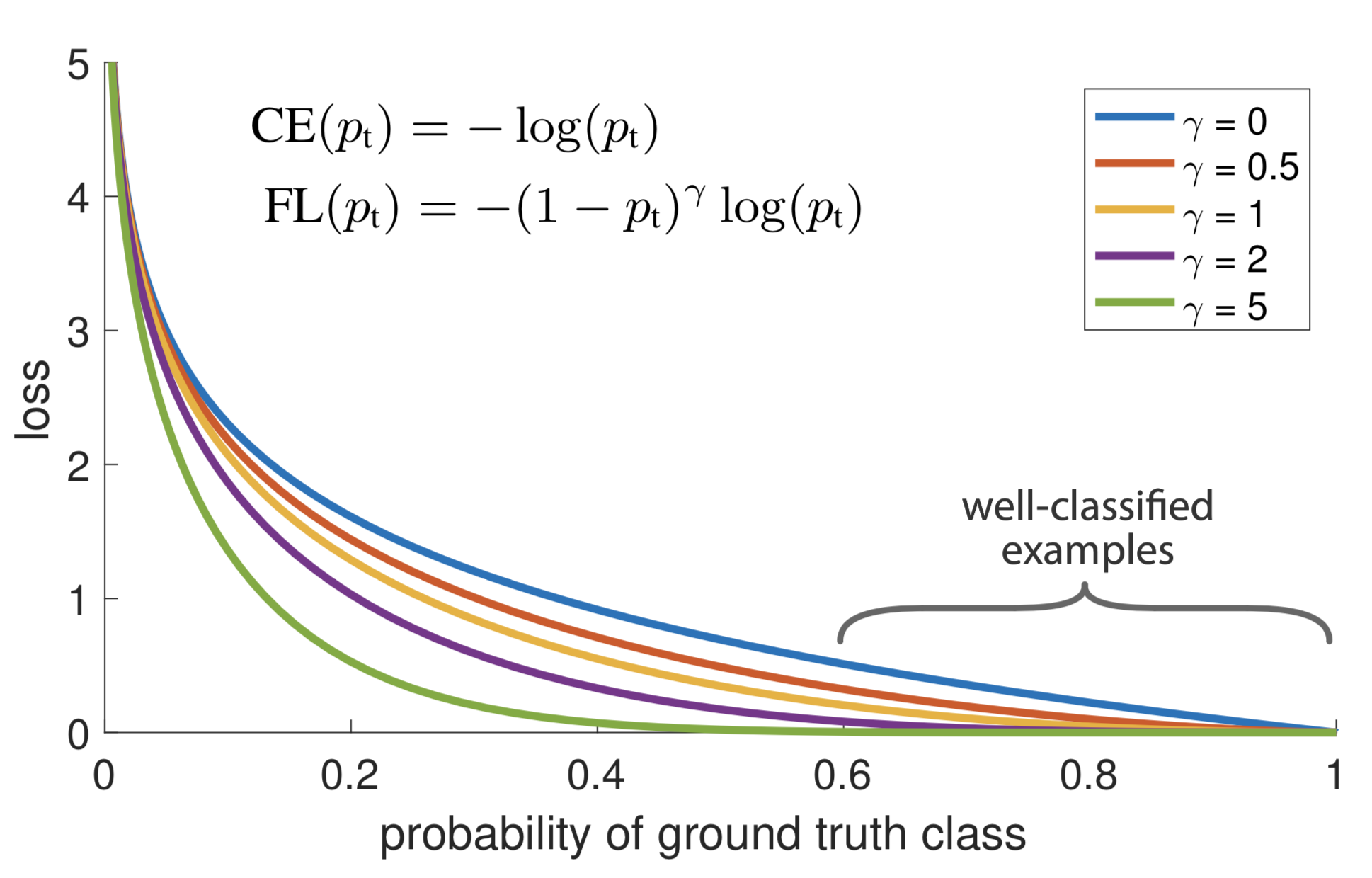
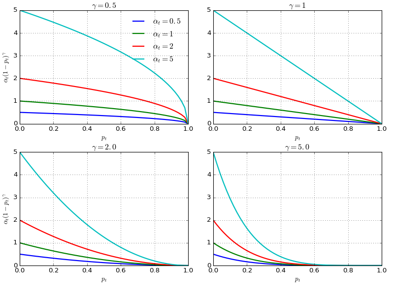
For a better control of the shape of the weighting function (see Fig. 10.), RetinaNet uses an $\alpha$-balanced variant of the focal loss, where $\alpha=0.25, \gamma=2$ works the best.

Featurized Image Pyramid

The featurized image pyramid (Lin et al., 2017) is the backbone network for RetinaNet. Following the same approach by image pyramid in SSD, featurized image pyramids provide a basic vision component for object detection at different scales.

The key idea of feature pyramid network is demonstrated in Fig. 11. The base structure contains a sequence of pyramid levels, each corresponding to one network stage. One stage contains multiple convolutional layers of the same size and the stage sizes are scaled down by a factor of 2. Let’s denote the last layer of the $i$-th stage as $C_i$.

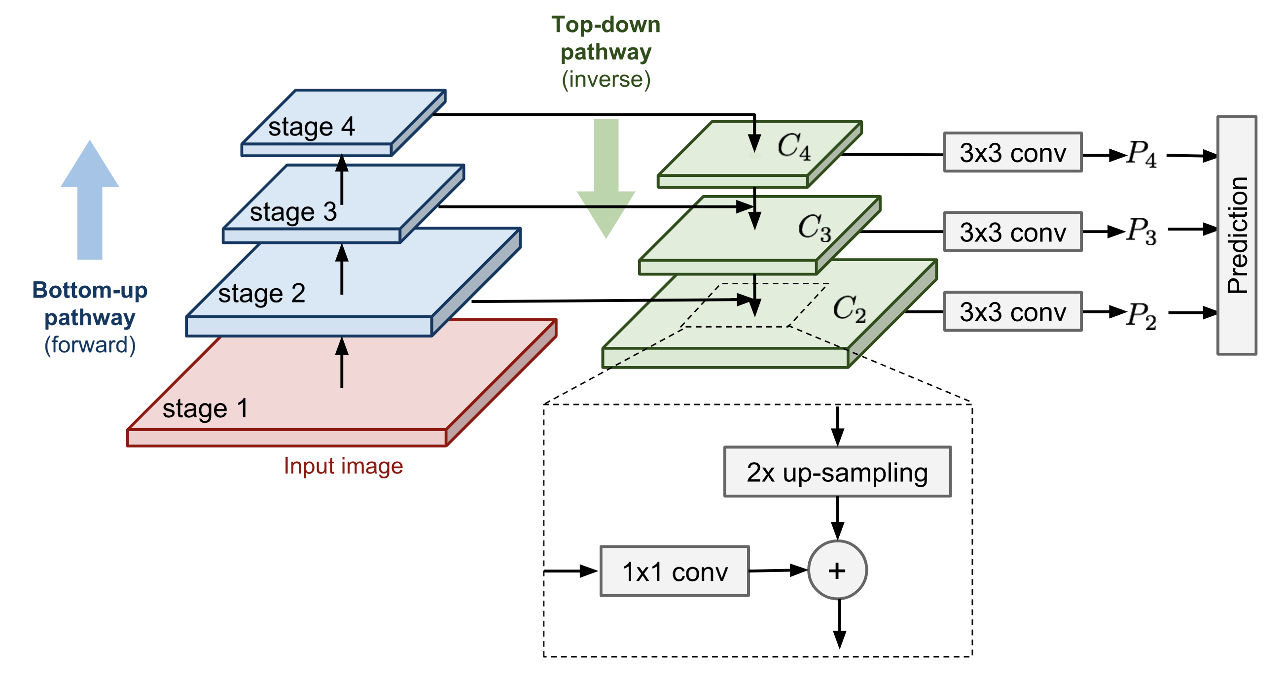
Two pathways connect conv layers:

• Bottom-up pathway is the normal feedforward computation.
• Top-down pathway goes in the inverse direction, adding coarse but semantically stronger feature maps back into the previous pyramid levels of a larger size via lateral connections.
  • First, the higher-level features are upsampled spatially coarser to be 2x larger. For image upscaling, the paper used nearest neighbor upsampling. While there are many image upscaling algorithms such as using deconv, adopting another image scaling method might or might not improve the performance of RetinaNet.
  • The larger feature map undergoes a 1x1 conv layer to reduce the channel dimension.
  • Finally, these two feature maps are merged by element-wise addition.
    
    The lateral connections only happen at the last layer in stages, denoted as $\{C_i\}$, and the process continues until the finest (largest) merged feature map is generated. The prediction is made out of every merged map after a 3x3 conv layer, $\{P_i\}$.

According to ablation studies, the importance rank of components of the featurized image pyramid design is as follows: 1x1 lateral connection > detect object across multiple layers > top-down enrichment > pyramid representation (compared to only check the finest layer).

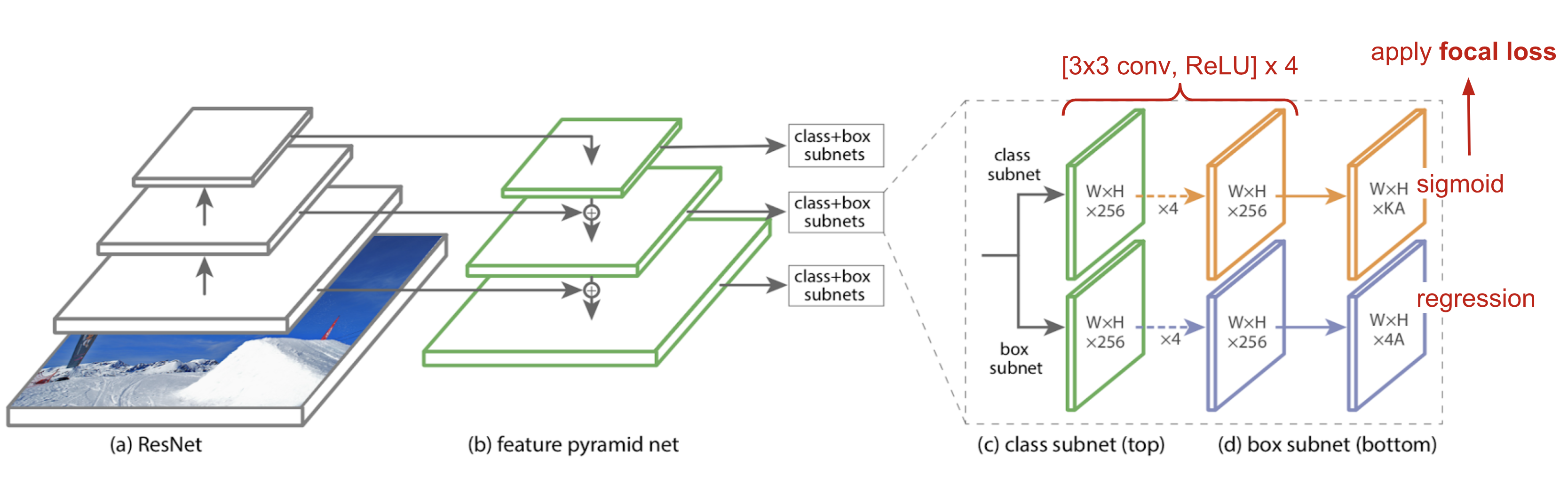
Model Architecture

The featurized pyramid is constructed on top of the ResNet architecture. Recall that ResNet has 5 conv blocks (= network stages / pyramid levels). The last layer of the $i$-th pyramid level, $C_i$, has resolution $2^i$ lower than the raw input dimension.

RetinaNet utilizes feature pyramid levels $P_3$ to $P_7$:

• $P_3$ to $P_5$ are computed from the corresponding ResNet residual stage from $C_3$ to $C_5$. They are connected by both top-down and bottom-up pathways.
• $P_6$ is obtained via a 3×3 stride-2 conv on top of $C_5$
• $P_7$ applies ReLU and a 3×3 stride-2 conv on $P_6$.

Adding higher pyramid levels on ResNet improves the performance for detecting large objects.

Same as in SSD, detection happens in all pyramid levels by making a prediction out of every merged feature map. Because predictions share the same classifier and the box regressor, they are all formed to have the same channel dimension d=256.

There are A=9 anchor boxes per level:

• The base size corresponds to areas of $32^2$ to $512^2$ pixels on $P_3$ to $P_7$ respectively. There are three size ratios, $\{2^0, 2^{1/3}, 2^{2/3}\}$.
• For each size, there are three aspect ratios {1/2, 1, 2}.

As usual, for each anchor box, the model outputs a class probability for each of $K$ classes in the classification subnet and regresses the offset from this anchor box to the nearest ground truth object in the box regression subnet. The classification subnet adopts the focal loss introduced above.

YOLOv3

YOLOv3 is created by applying a bunch of design tricks on YOLOv2. The changes are inspired by recent advances in the object detection world.

Here are a list of changes:

1. Logistic regression for confidence scores: YOLOv3 predicts an confidence score for each bounding box using logistic regression, while YOLO and YOLOv2 uses sum of squared errors for classification terms (see the loss function above). Linear regression of offset prediction leads to a decrease in mAP.

2. No more softmax for class prediction: When predicting class confidence, YOLOv3 uses multiple independent logistic classifier for each class rather than one softmax layer. This is very helpful especially considering that one image might have multiple labels and not all the labels are guaranteed to be mutually exclusive.

3. Darknet + ResNet as the base model: The new Darknet-53 still relies on successive 3x3 and 1x1 conv layers, just like the original dark net architecture, but has residual blocks added.

4. Multi-scale prediction: Inspired by image pyramid, YOLOv3 adds several conv layers after the base feature extractor model and makes prediction at three different scales among these conv layers. In this way, it has to deal with many more bounding box candidates of various sizes overall.

5. Skip-layer concatenation: YOLOv3 also adds cross-layer connections between two prediction layers (except for the output layer) and earlier finer-grained feature maps. The model first up-samples the coarse feature maps and then merges it with the previous features by concatenation. The combination with finer-grained information makes it better at detecting small objects.

Interestingly, focal loss does not help YOLOv3, potentially it might be due to the usage of $\lambda_\text{noobj}$ and $\lambda_\text{coord}$ — they increase the loss from bounding box location predictions and decrease the loss from confidence predictions for background boxes.

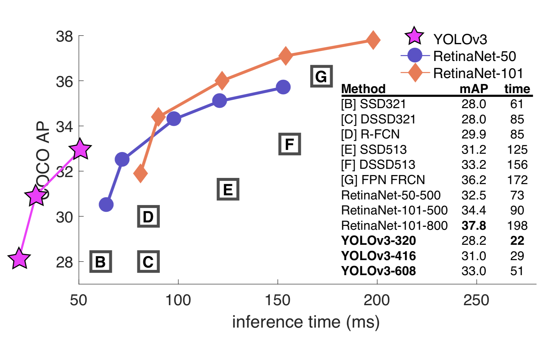
Overall YOLOv3 performs better and faster than SSD, and worse than RetinaNet but 3.8x faster.

Cited as:

@article{weng2018detection4,
  title   = "Object Detection Part 4: Fast Detection Models",
  author  = "Weng, Lilian",
  journal = "lilianweng.github.io",
  year    = "2018",
  url     = "https://lilianweng.github.io/posts/2018-12-27-object-recognition-part-4/"
}

Reference

[1] Joseph Redmon, et al. “You only look once: Unified, real-time object detection.” CVPR 2016.

[2] Joseph Redmon and Ali Farhadi. “YOLO9000: Better, Faster, Stronger.” CVPR 2017.

[3] Joseph Redmon, Ali Farhadi. “YOLOv3: An incremental improvement.”.

[4] Wei Liu et al. “SSD: Single Shot MultiBox Detector.” ECCV 2016.

[5] Tsung-Yi Lin, et al. “Feature Pyramid Networks for Object Detection.” CVPR 2017.

[6] Tsung-Yi Lin, et al. “Focal Loss for Dense Object Detection.” IEEE transactions on pattern analysis and machine intelligence, 2018.

[7] “What’s new in YOLO v3?” by Ayoosh Kathuria on “Towards Data Science”, Apr 23, 2018.