Part 1 of the “Object Detection for Dummies” series introduced: (1) the concept of image gradient vector and how HOG algorithm summarizes the information across all the gradient vectors in one image; (2) how the image segmentation algorithm works to detect regions that potentially contain objects; (3) how the Selective Search algorithm refines the outcomes of image segmentation for better region proposal.

In Part 2, we are about to find out more on the classic convolution neural network architectures for image classification. They lay the foundation for further progress on the deep learning models for object detection. Go check Part 3 if you want to learn more on R-CNN and related models.

Links to all the posts in the series: [Part 1] [Part 2] [Part 3] [Part 4].

CNN for Image Classification

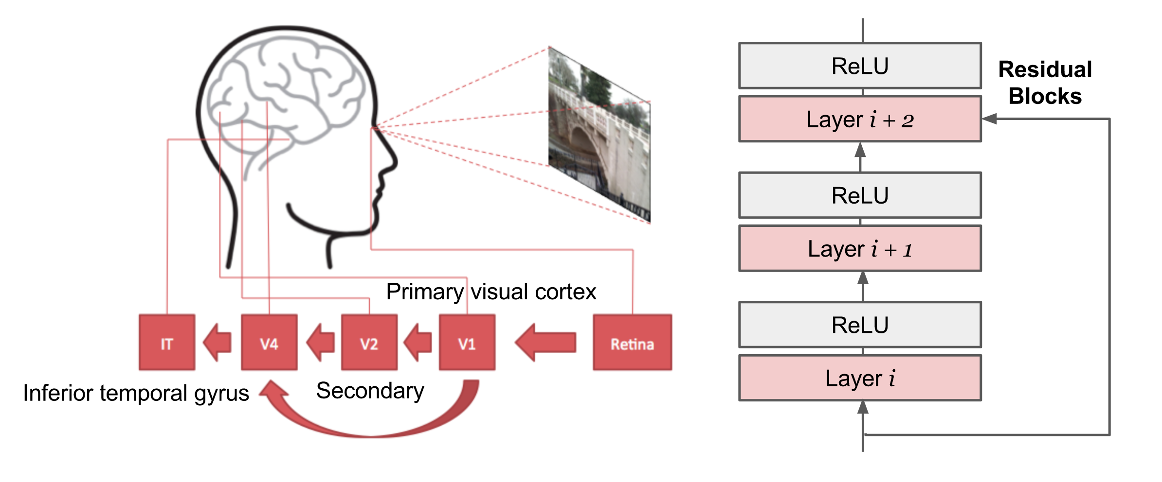
CNN, short for “Convolutional Neural Network”, is the go-to solution for computer vision problems in the deep learning world. It was, to some extent, inspired by how human visual cortex system works.

Convolution Operation

I strongly recommend this guide to convolution arithmetic, which provides a clean and solid explanation with tons of visualizations and examples. Here let’s focus on two-dimensional convolution as we are working with images in this post.

In short, convolution operation slides a predefined kernel (also called “filter”) on top of the input feature map (matrix of image pixels), multiplying and adding the values of the kernel and partial input features to generate the output. The values form an output matrix, as usually, the kernel is much smaller than the input image.

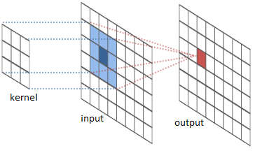
Figure 2 showcases two real examples of how to convolve a 3x3 kernel over a 5x5 2D matrix of numeric values to generate a 3x3 matrix. By controlling the padding size and the stride length, we can generate an output matrix of a certain size.

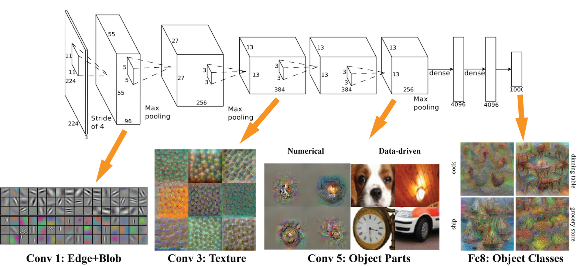
AlexNet (Krizhevsky et al, 2012)

• 5 convolution [+ optional max pooling] layers + 2 MLP layers + 1 LR layer
• Use data augmentation techniques to expand the training dataset, such as image translations, horizontal reflections, and patch extractions.

VGG (Simonyan and Zisserman, 2014)

• The network is considered as “very deep” at its time; 19 layers
• The architecture is extremely simplified with only 3x3 convolutional layers and 2x2 pooling layers. The stacking of small filters simulates a larger filter with fewer parameters.

ResNet (He et al., 2015)

• The network is indeed very deep; 152 layers of simple architecture.
• Residual Block: Some input of a certain layer can be passed to the component two layers later. Residual blocks are essential for keeping a deep network trainable and eventually work. Without residual blocks, the training loss of a plain network does not monotonically decrease as the number of layers increases due to vanishing and exploding gradients.

Evaluation Metrics: mAP

A common evaluation metric used in many object recognition and detection tasks is “mAP”, short for “mean average precision”. It is a number from 0 to 100; higher value is better.

• Combine all detections from all test images to draw a precision-recall curve (PR curve) for each class; The “average precision” (AP) is the area under the PR curve.
• Given that target objects are in different classes, we first compute AP separately for each class, and then average over classes.
• A detection is a true positive if it has “intersection over union” (IoU) with a ground-truth box greater than some threshold (usually 0.5; if so, the metric is “mAP@0.5”)

Deformable Parts Model

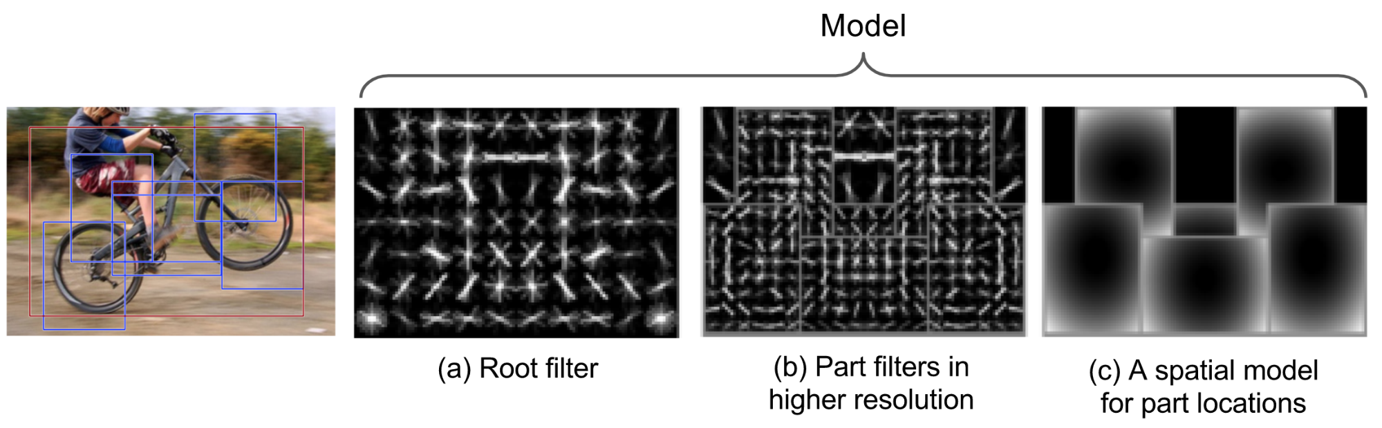
The Deformable Parts Model (DPM) (Felzenszwalb et al., 2010) recognizes objects with a mixture graphical model (Markov random fields) of deformable parts. The model consists of three major components:

1. A coarse root filter defines a detection window that approximately covers an entire object. A filter specifies weights for a region feature vector.
2. Multiple part filters that cover smaller parts of the object. Parts filters are learned at twice resolution of the root filter.
3. A spatial model for scoring the locations of part filters relative to the root.

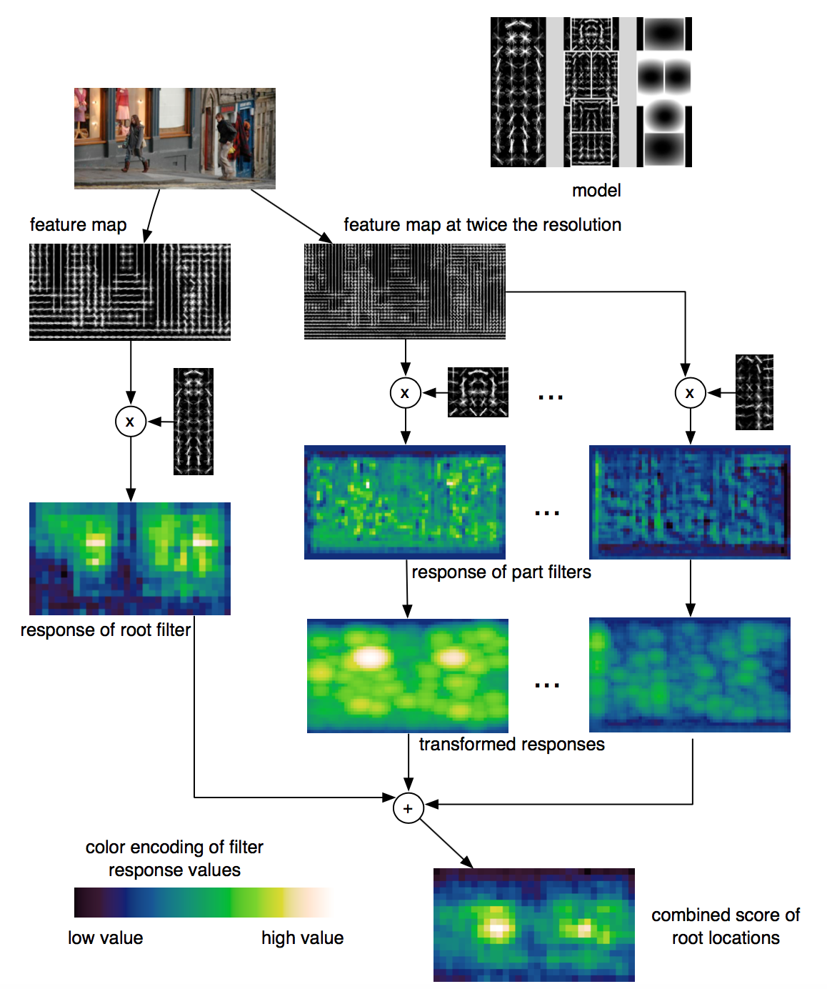
The quality of detecting an object is measured by the score of filters minus the deformation costs. The matching score $f$, in laymen’s terms, is:

in which,

• $x$ is an image with a specified position and scale;
• $y$ is a sub region of $x$.
• $\beta_\text{root}$ is the root filter.
• $\beta_\text{part}$ is one part filter.
• cost() measures the penalty of the part deviating from its ideal location relative to the root.

The basic score model is the dot product between the filter $\beta$ and the region feature vector $\Phi(x)$: $f(\beta, x) = \beta \cdot \Phi(x)$. The feature set $\Phi(x)$ can be defined by HOG or other similar algorithms.

A root location with high score detects a region with high chances to contain an object, while the locations of the parts with high scores confirm a recognized object hypothesis. The paper adopted latent SVM to model the classifier.

The author later claimed that DPM and CNN models are not two distinct approaches to object recognition. Instead, a DPM model can be formulated as a CNN by unrolling the DPM inference algorithm and mapping each step to an equivalent CNN layer. (Check the details in Girshick et al., 2015!)

Overfeat

Overfeat [paper][code] is a pioneer model of integrating the object detection, localization and classification tasks all into one convolutional neural network. The main idea is to (i) do image classification at different locations on regions of multiple scales of the image in a sliding window fashion, and (ii) predict the bounding box locations with a regressor trained on top of the same convolution layers.

The Overfeat model architecture is very similar to AlexNet. It is trained as follows:

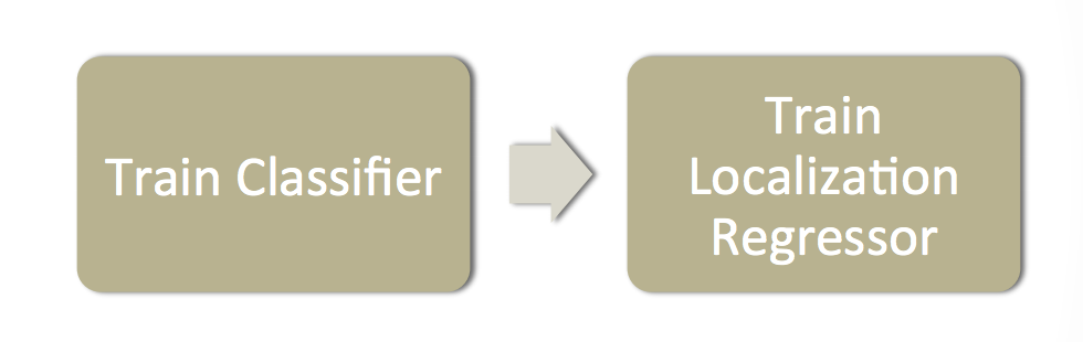
1. Train a CNN model (similar to AlexNet) on the image classification task.
2. Then, we replace the top classifier layers by a regression network and train it to predict object bounding boxes at each spatial location and scale. The regressor is class-specific, each generated for one image class.
   • Input: Images with classification and bounding box.
   • Output: $(x_\text{left}, x_\text{right}, y_\text{top}, y_\text{bottom})$, 4 values in total, representing the coordinates of the bounding box edges.
   • Loss: The regressor is trained to minimize $l2$ norm between generated bounding box and the ground truth for each training example.

At the detection time,

1. Perform classification at each location using the pretrained CNN model.
2. Predict object bounding boxes on all classified regions generated by the classifier.
3. Merge bounding boxes with sufficient overlap from localization and sufficient confidence of being the same object from the classifier.

Cited as:

@article{weng2017detection2,
  title   = "Object Detection for Dummies Part 2: CNN, DPM and Overfeat",
  author  = "Weng, Lilian",
  journal = "lilianweng.github.io",
  year    = "2017",
  url     = "https://lilianweng.github.io/posts/2017-12-15-object-recognition-part-2/"
}

Reference

[1] Vincent Dumoulin and Francesco Visin. “A guide to convolution arithmetic for deep learning.” arXiv preprint arXiv:1603.07285 (2016).

[2] Haohan Wang, Bhiksha Raj, and Eric P. Xing. “On the Origin of Deep Learning.” arXiv preprint arXiv:1702.07800 (2017).

[3] Pedro F. Felzenszwalb, Ross B. Girshick, David McAllester, and Deva Ramanan. “Object detection with discriminatively trained part-based models.” IEEE transactions on pattern analysis and machine intelligence 32, no. 9 (2010): 1627-1645.

[4] Ross B. Girshick, Forrest Iandola, Trevor Darrell, and Jitendra Malik. “Deformable part models are convolutional neural networks.” In Proc. IEEE Conf. on Computer Vision and Pattern Recognition (CVPR), pp. 437-446. 2015.

[5] Sermanet, Pierre, David Eigen, Xiang Zhang, Michaël Mathieu, Rob Fergus, and Yann LeCun. “OverFeat: Integrated Recognition, Localization and Detection using Convolutional Networks” arXiv preprint arXiv:1312.6229 (2013).