(The post was originated from my talk for WiMLDS x Fintech meetup hosted by Affirm.)
I believe many of you have watched or heard of the games between AlphaGo and professional Go player Lee Sedol in 2016. Lee has the highest rank of nine dan and many world championships. No doubt, he is one of the best Go players in the world, but he lost by 1-4 in this series versus AlphaGo. Before this, Go was considered to be an intractable game for computers to master, as its simple rules lay out an exponential number of variations in the board positions, many more than what in Chess. This event surely highlighted 2016 as a big year for AI. Because of AlphaGo, much attention has been attracted to the progress of AI.
Meanwhile, many companies are spending resources on pushing the edges of AI applications, that indeed have the potential to change or even revolutionize how we are gonna live. Familiar examples include self-driving cars, chatbots, home assistant devices and many others. One of the secret receipts behind the progress we have had in recent years is deep learning.
Why Does Deep Learning Work Now?
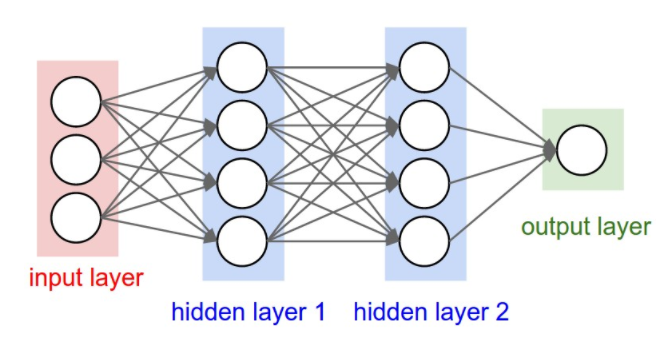
Deep learning models, in simple words, are large and deep artificial neural nets. A neural network (“NN”) can be well presented in a directed acyclic graph: the input layer takes in signal vectors; one or multiple hidden layers process the outputs of the previous layer. The initial concept of a neural network can be traced back to more than half a century ago. But why does it work now? Why do people start talking about them all of a sudden?
The reason is surprisingly simple:
- We have a lot more data.
- We have much powerful computers.
A large and deep neural network has many more layers + many more nodes in each layer, which results in exponentially many more parameters to tune. Without enough data, we cannot learn parameters efficiently. Without powerful computers, learning would be too slow and insufficient.
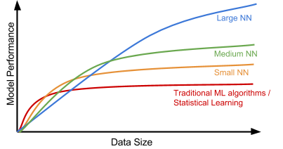
Here is an interesting plot presenting the relationship between the data scale and the model performance, proposed by Andrew Ng in his “Nuts and Bolts of Applying Deep Learning” talk. On a small dataset, traditional algorithms (Regression, Random Forests, SVM, GBM, etc.) or statistical learning does a great job, but once the data scale goes up to the sky, the large NN outperforms others. Partially because compared to a traditional ML model, a neural network model has many more parameters and has the capability to learn complicated nonlinear patterns. Thus we expect the model to pick the most helpful features by itself without too much expert-involved manual feature engineering.
Deep Learning Models
Next, let’s go through a few classical deep learning models.
Convolutional Neural Network
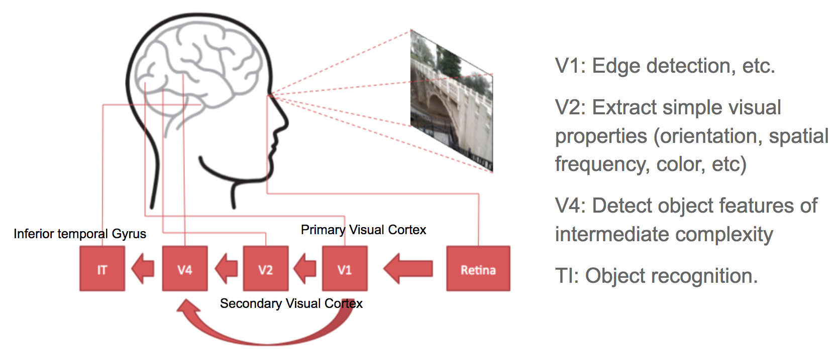
Convolutional neural networks, short for “CNN”, is a type of feed-forward artificial neural networks, in which the connectivity pattern between its neurons is inspired by the organization of the visual cortex system. The primary visual cortex (V1) does edge detection out of the raw visual input from the retina. The secondary visual cortex (V2), also called prestriate cortex, receives the edge features from V1 and extracts simple visual properties such as orientation, spatial frequency, and color. The visual area V4 handles more complicated object attributes. All the processed visual features flow into the final logic unit, inferior temporal gyrus (IT), for object recognition. The shortcut between V1 and V4 inspires a special type of CNN with connections between non-adjacent layers: Residual Net (He, et al. 2016) containing “Residual Block” which supports some input of one layer to be passed to the component two layers later.
Convolution is a mathematical term, here referring to an operation between two matrices. The convolutional layer has a fixed small matrix defined, also called kernel or filter. As the kernel is sliding, or convolving, across the matrix representation of the input image, it is computing the element-wise multiplication of the values in the kernel matrix and the original image values. Specially designed kernels can process images for common purposes like blurring, sharpening, edge detection and many others, fast and efficiently.
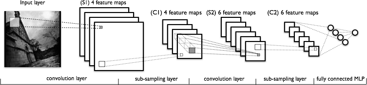
Convolutional and pooling (or “sub-sampling” in Fig. 4) layers act like the V1, V2 and V4 visual cortex units, responding to feature extraction. The object recognition reasoning happens in the later fully-connected layers which consume the extracted features.
Recurrent Neural Network
A sequence model is usually designed to transform an input sequence into an output sequence that lives in a different domain. Recurrent neural network, short for “RNN”, is suitable for this purpose and has shown tremendous improvement in problems like handwriting recognition, speech recognition, and machine translation (Sutskever et al. 2011, Liwicki et al. 2007).
A recurrent neural network model is born with the capability to process long sequential data and to tackle tasks with context spreading in time. The model processes one element in the sequence at one time step. After computation, the newly updated unit state is passed down to the next time step to facilitate the computation of the next element. Imagine the case when an RNN model reads all the Wikipedia articles, character by character, and then it can predict the following words given the context.
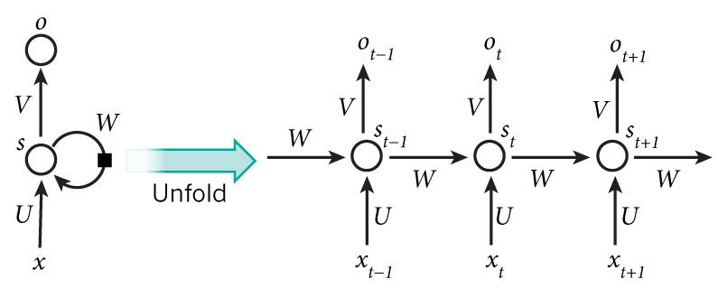
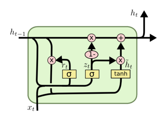
However, simple perceptron neurons that linearly combine the current input element and the last unit state may easily lose the long-term dependencies. For example, we start a sentence with “Alice is working at …” and later after a whole paragraph, we want to start the next sentence with “She” or “He” correctly. If the model forgets the character’s name “Alice”, we can never know. To resolve the issue, researchers created a special neuron with a much more complicated internal structure for memorizing long-term context, named “Long-short term memory (LSTM)” cell. It is smart enough to learn for how long it should memorize the old information, when to forget, when to make use of the new data, and how to combine the old memory with new input. This introduction is so well written that I recommend everyone with interest in LSTM to read it. It has been officially promoted in the Tensorflow documentation ;-)
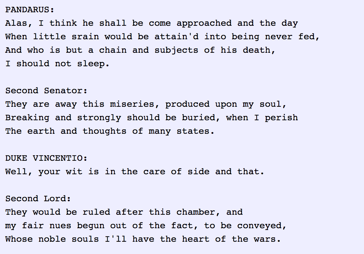
To demonstrate the power of RNNs, Andrej Karpathy built a character-based language model using RNN with LSTM cells. Without knowing any English vocabulary beforehand, the model could learn the relationship between characters to form words and then the relationship between words to form sentences. It could achieve a decent performance even without a huge set of training data.
RNN: Sequence-to-Sequence Model
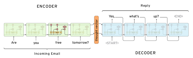
The sequence-to-sequence model is an extended version of RNN, but its application field is distinguishable enough that I would like to list it in a separated section. Same as RNN, a sequence-to-sequence model operates on sequential data, but particularly it is commonly used to develop chatbots or personal assistants, both generating meaningful response for input questions. A sequence-to-sequence model consists of two RNNs, encoder and decoder. The encoder learns the contextual information from the input words and then hands over the knowledge to the decoder side through a “context vector” (or “thought vector”, as shown in Fig 8.). Finally, the decoder consumes the context vector and generates proper responses.
Autoencoders
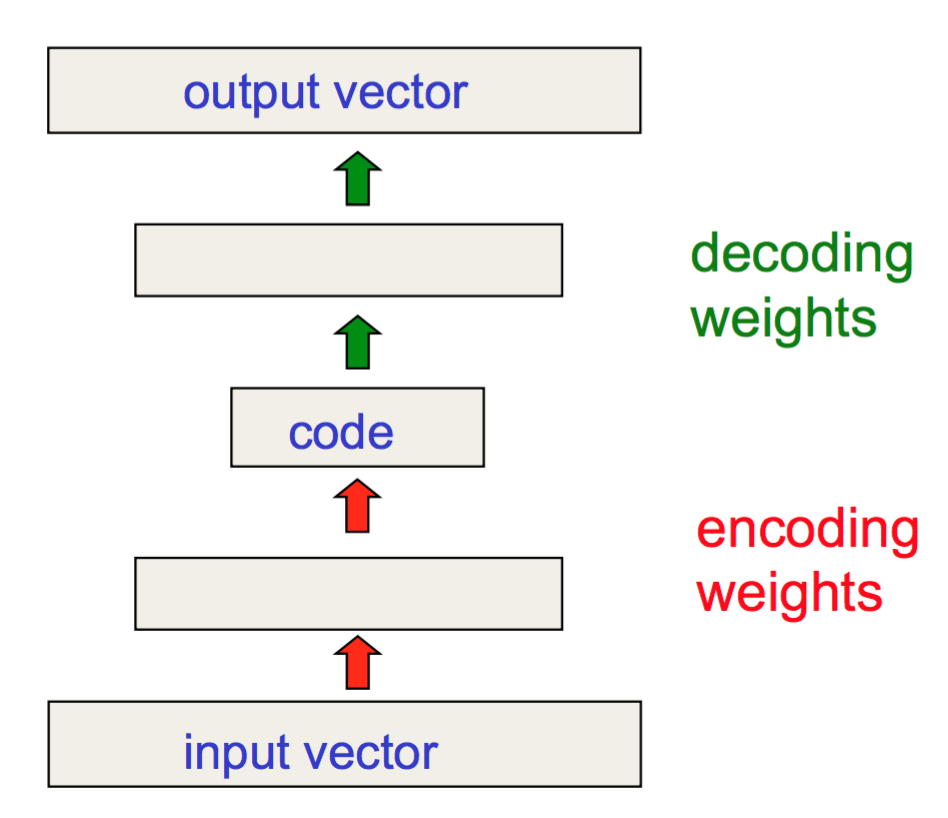
Different from the previous models, autoencoders are for unsupervised learning. It is designed to learn a low-dimensional representation of a high-dimensional data set, similar to what Principal Components Analysis (PCA) does. The autoencoder model tries to learn an approximation function $ f(x) \approx x $ to reproduce the input data. However, it is restricted by a bottleneck layer in the middle with a very small number of nodes. With limited capacity, the model is forced to form a very efficient encoding of the data, that is essentially the low-dimensional code we learned.
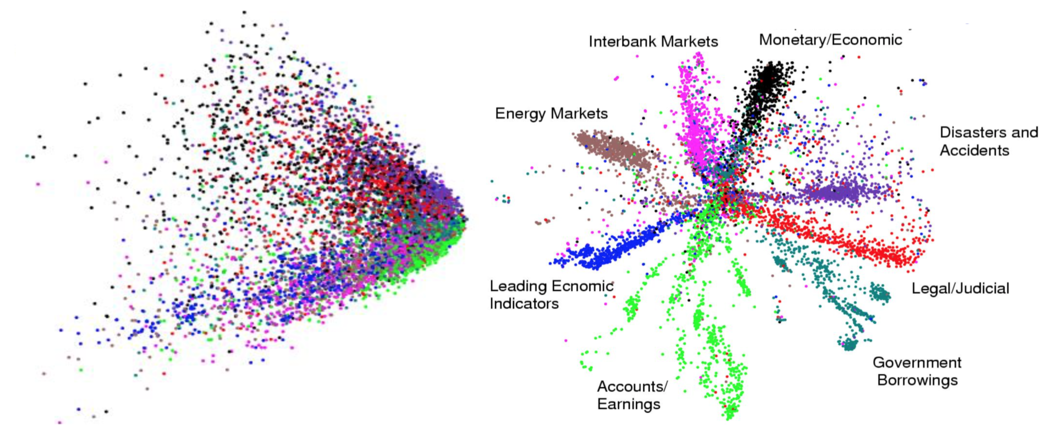
Hinton and Salakhutdinov used autoencoders to compress documents on a variety of topics. As shown in Fig 10, when both PCA and autoencoder were applied to reduce the documents onto two dimensions, autoencoder demonstrated a much better outcome. With the help of autoencoder, we can do efficient data compression to speed up the information retrieval including both documents and images.
Reinforcement (Deep) Learning
Since I started my post with AlphaGo, let us dig a bit more on why AlphaGo worked out. Reinforcement learning (“RL”) is one of the secrets behind its success. RL is a subfield of machine learning which allows machines and software agents to automatically determine the optimal behavior within a given context, with a goal to maximize the long-term performance measured by a given metric.
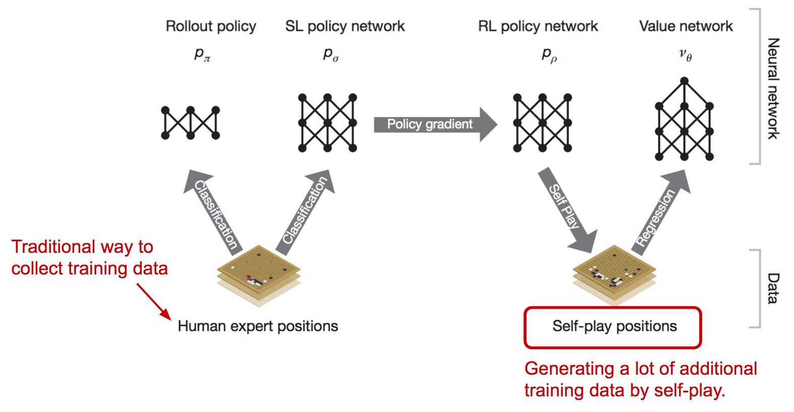
The AlphaGo system starts with a supervised learning process to train a fast rollout policy and a policy network, relying on the manually curated training dataset of professional players’ games. It learns what is the best strategy given the current position on the game board. Then it applies reinforcement learning by setting up self-play games. The RL policy network gets improved when it wins more and more games against previous versions of the policy network. In the self-play stage, AlphaGo becomes stronger and stronger by playing against itself without requiring additional external training data.
Generative Adversarial Network
Generative adversarial network, short for “GAN”, is a type of deep generative models. GAN is able to create new examples after learning through the real data. It is consist of two models competing against each other in a zero-sum game framework. The famous deep learning researcher Yann LeCun gave it a super high praise: Generative Adversarial Network is the most interesting idea in the last ten years in machine learning. (See the Quora question: “What are some recent and potentially upcoming breakthroughs in deep learning?”)
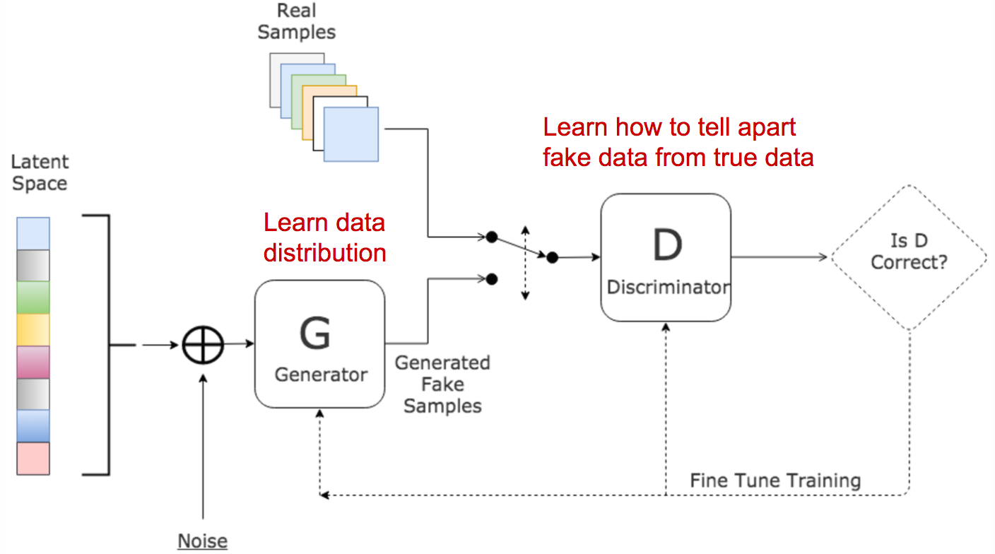
In the original GAN paper, GAN was proposed to generate meaningful images after learning from real photos. It comprises two independent models: the Generator and the Discriminator. The generator produces fake images and sends the output to the discriminator model. The discriminator works like a judge, as it is optimized for identifying the real photos from the fake ones. The generator model is trying hard to cheat the discriminator while the judge is trying hard not to be cheated. This interesting zero-sum game between these two models motivates both to develop their designed skills and improve their functionalities. Eventually, we take the generator model for producing new images.
Toolkits and Libraries
After learning all these models, you may start wondering how you can implement the models and use them for real. Fortunately, we have many open source toolkits and libraries for building deep learning models. Tensorflow is fairly new but has attracted a lot of popularity. It turns out, TensorFlow was the most forked Github project of 2015. All that happened in a period of 2 months after its release in Nov 2015.

How to Learn?
If you are very new to the field and willing to devote some time to studying deep learning in a more systematic way, I would recommend you to start with the book Deep Learning by Ian Goodfellow, Yoshua Bengio, and Aaron Courville. The Coursera course “Neural Networks for Machine Learning” by Geoffrey Hinton (Godfather of deep learning!). The content for the course was prepared around 2006, pretty old, but it helps you build up a solid foundation for understanding deep learning models and expedite further exploration.
Meanwhile, maintain your curiosity and passion. The field is making progress every day. Even classical or widely adopted deep learning models may just have been proposed 1-2 years ago. Reading academic papers can help you learn stuff in depth and keep up with the cutting-edge findings.
Useful resources
- Google Scholar: http://scholar.google.com
- arXiv cs section: https://arxiv.org/list/cs/recent
- Unsupervised Feature Learning and Deep Learning Tutorial
- Tensorflow Tutorials
- Data Science Weekly
- KDnuggets
- Tons of blog posts and online tutorials
- Related Cousera courses
- awesome-deep-learning-papers
Blog posts mentioned
- Explained Visually: Image Kernels
- Understanding LSTM Networks
- The Unreasonable Effectiveness of Recurrent Neural Networks
- Computer, respond to this email.
Interesting blogs worthy of checking
Papers mentioned
[1] He, Kaiming, et al. “Deep residual learning for image recognition.” Proc. IEEE Conf. on computer vision and pattern recognition. 2016.
[2] Wang, Haohan, Bhiksha Raj, and Eric P. Xing. “On the Origin of Deep Learning.” arXiv preprint arXiv:1702.07800, 2017.
[3] Sutskever, Ilya, James Martens, and Geoffrey E. Hinton. “Generating text with recurrent neural networks.” Proc. of the 28th Intl. Conf. on Machine Learning (ICML). 2011.
[4] Liwicki, Marcus, et al. “A novel approach to on-line handwriting recognition based on bidirectional long short-term memory networks.” Proc. of 9th Intl. Conf. on Document Analysis and Recognition. 2007.
[5] LeCun, Yann, Yoshua Bengio, and Geoffrey Hinton. “Deep learning.” Nature 521.7553 (2015): 436-444.
[6] Hochreiter, Sepp, and Jurgen Schmidhuber. “Long short-term memory.” Neural computation 9.8 (1997): 1735-1780.
[7] Cho, Kyunghyun. et al. “Learning phrase representations using RNN encoder-decoder for statistical machine translation.” Proc. Conference on Empirical Methods in Natural Language Processing 1724–1734 (2014).
[8] Hinton, Geoffrey E., and Ruslan R. Salakhutdinov. “Reducing the dimensionality of data with neural networks.” science 313.5786 (2006): 504-507.
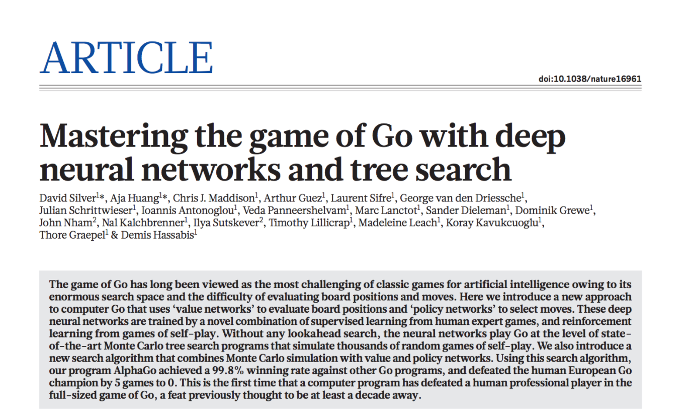
[9] Silver, David, et al. “Mastering the game of Go with deep neural networks and tree search.” Nature 529.7587 (2016): 484-489.
[10] Goodfellow, Ian, et al. “Generative adversarial nets.” NIPS, 2014.