This is a tutorial for how to build a recurrent neural network using Tensorflow to predict stock market prices. The full working code is available in github.com/lilianweng/stock-rnn. If you don’t know what is recurrent neural network or LSTM cell, feel free to check my previous post.

One thing I would like to emphasize that because my motivation for writing this post is more on demonstrating how to build and train an RNN model in Tensorflow and less on solve the stock prediction problem, I didn’t try hard on improving the prediction outcomes. You are more than welcome to take my code as a reference point and add more stock prediction related ideas to improve it. Enjoy!

Overview of Existing Tutorials

There are many tutorials on the Internet, like:

• A noob’s guide to implementing RNN-LSTM using Tensorflow
• TensorFlow RNN Tutorial
• LSTM by Example using Tensorflow
• How to build a Recurrent Neural Network in TensorFlow
• RNNs in Tensorflow, a Practical Guide and Undocumented Features
• Sequence prediction using recurrent neural networks(LSTM) with TensorFlow
• Anyone Can Learn To Code an LSTM-RNN in Python
• How to do time series prediction using RNNs, TensorFlow and Cloud ML Engine

Despite all these existing tutorials, I still want to write a new one mainly for three reasons:

1. Early tutorials cannot cope with the new version any more, as Tensorflow is still under development and changes on API interfaces are being made fast.
2. Many tutorials use synthetic data in the examples. Well, I would like to play with the real world data.
3. Some tutorials assume that you have known something about Tensorflow API beforehand, which makes the reading a bit difficult.

After reading a bunch of examples, I would like to suggest taking the official example on Penn Tree Bank (PTB) dataset as your starting point. The PTB example showcases a RNN model in a pretty and modular design pattern, but it might prevent you from easily understanding the model structure. Hence, here I will build up the graph in a very straightforward manner.

The Goal

I will explain how to build an RNN model with LSTM cells to predict the prices of S&P500 index. The dataset can be downloaded from Yahoo! Finance ^GSPC. In the following example, I used S&P 500 data from Jan 3, 1950 (the maximum date that Yahoo! Finance is able to trace back to) to Jun 23, 2017. The dataset provides several price points per day. For simplicity, we will only use the daily close prices for prediction. Meanwhile, I will demonstrate how to use TensorBoard for easily debugging and model tracking.

As a quick recap: the recurrent neural network (RNN) is a type of artificial neural network with self-loop in its hidden layer(s), which enables RNN to use the previous state of the hidden neuron(s) to learn the current state given the new input. RNN is good at processing sequential data. Long short-term memory (LSTM) cell is a specially designed working unit that helps RNN better memorize the long-term context.

For more information in depth, please read my previous post or this awesome post.

Data Preparation

The stock prices is a time series of length $N$, defined as $p_0, p_1, \dots, p_{N-1}$ in which $p_i$ is the close price on day $i$, $0 \le i < N$. Imagine that we have a sliding window of a fixed size $w$ (later, we refer to this as input_size) and every time we move the window to the right by size $w$, so that there is no overlap between data in all the sliding windows.

The RNN model we are about to build has LSTM cells as basic hidden units. We use values from the very beginning in the first sliding window $W_0$ to the window $W_t$ at time $t$:

to predict the prices in the following window $w_{t+1}$:

$$ W_{t+1} = (p_{(t+1)w}, p_{(t+1)w+1}, \dots, p_{(t+2)w-1}) $$

Essentially we try to learn an approximation function, $f(W_0, W_1, \dots, W_t) \approx W_{t+1}$.

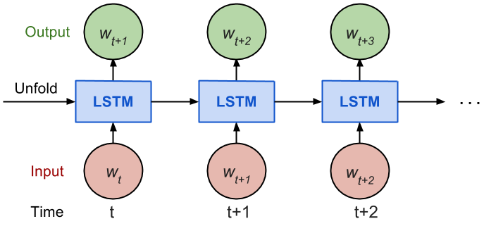
Considering how back propagation through time (BPTT) works, we usually train RNN in a “unrolled” version so that we don’t have to do propagation computation too far back and save the training complication.

Here is the explanation on num_steps from Tensorflow’s tutorial:

By design, the output of a recurrent neural network (RNN) depends on arbitrarily distant inputs. Unfortunately, this makes backpropagation computation difficult. In order to make the learning process tractable, it is common practice to create an “unrolled” version of the network, which contains a fixed number (num_steps) of LSTM inputs and outputs. The model is then trained on this finite approximation of the RNN. This can be implemented by feeding inputs of length num_steps at a time and performing a backward pass after each such input block.

The sequence of prices are first split into non-overlapped small windows. Each contains input_size numbers and each is considered as one independent input element. Then any num_steps consecutive input elements are grouped into one training input, forming an “un-rolled” version of RNN for training on Tensorfow. The corresponding label is the input element right after them.

For instance, if input_size=3 and num_steps=2, my first few training examples would look like:

Here is the key part for formatting the data:

seq = [np.array(seq[i * self.input_size: (i + 1) * self.input_size]) 
       for i in range(len(seq) // self.input_size)]

# Split into groups of `num_steps`
X = np.array([seq[i: i + self.num_steps] for i in range(len(seq) - self.num_steps)])
y = np.array([seq[i + self.num_steps] for i in range(len(seq) - self.num_steps)])

The complete code of data formatting is here.

Train / Test Split

Since we always want to predict the future, we take the latest 10% of data as the test data.

Normalization

The S&P 500 index increases in time, bringing about the problem that most values in the test set are out of the scale of the train set and thus the model has to predict some numbers it has never seen before. Sadly and unsurprisingly, it does a tragic job. See 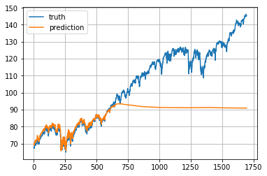Fig. 3.

To solve the out-of-scale issue, I normalize the prices in each sliding window. The task becomes predicting the relative change rates instead of the absolute values. In a normalized sliding window $W’_t$ at time $t$, all the values are divided by the last unknown price—the last price in $W_{t-1}$:

$$ W’_t = (\frac{p_{tw}}{p_{tw-1}}, \frac{p_{tw+1}}{p_{tw-1}}, \dots, \frac{p_{(t+1)w-1}}{p_{tw-1}}) $$

Here is a data archive stock-data-lilianweng.tar.gz of S & P 500 stock prices I crawled up to Jul, 2017. Feel free to play with it :)

Model Construction

Definitions

• lstm_size: number of units in one LSTM layer.
• num_layers: number of stacked LSTM layers.
• keep_prob: percentage of cell units to keep in the dropout operation.
• init_learning_rate: the learning rate to start with.
• learning_rate_decay: decay ratio in later training epochs.
• init_epoch: number of epochs using the constant init_learning_rate.
• max_epoch: total number of epochs in training
• input_size: size of the sliding window / one training data point
• batch_size: number of data points to use in one mini-batch.

The LSTM model has num_layers stacked LSTM layer(s) and each layer contains lstm_size number of LSTM cells. Then a dropout mask with keep probability keep_prob is applied to the output of every LSTM cell. The goal of dropout is to remove the potential strong dependency on one dimension so as to prevent overfitting.

The training requires max_epoch epochs in total; an epoch is a single full pass of all the training data points. In one epoch, the training data points are split into mini-batches of size batch_size. We send one mini-batch to the model for one BPTT learning. The learning rate is set to init_learning_rate during the first init_epoch epochs and then decay by $\times$ learning_rate_decay during every succeeding epoch.

# Configuration is wrapped in one object for easy tracking and passing.
class RNNConfig():
    input_size=1
    num_steps=30
    lstm_size=128
    num_layers=1
    keep_prob=0.8
    batch_size = 64
    init_learning_rate = 0.001
    learning_rate_decay = 0.99
    init_epoch = 5
    max_epoch = 50

config = RNNConfig()

Define Graph

A tf.Graph is not attached to any real data. It defines the flow of how to process the data and how to run the computation. Later, this graph can be fed with data within a tf.session and at this moment the computation happens for real.

— Let’s start going through some code —

(1) Initialize a new graph first.

import tensorflow as tf
tf.reset_default_graph()
lstm_graph = tf.Graph()

(2) How the graph works should be defined within its scope.

with lstm_graph.as_default():

(3) Define the data required for computation. Here we need three input variables, all defined as tf.placeholder because we don’t know what they are at the graph construction stage.

• inputs: the training data X, a tensor of shape (# data examples, num_steps, input_size); the number of data examples is unknown, so it is None. In our case, it would be batch_size in training session. Check the input format example if confused.
• targets: the training label y, a tensor of shape (# data examples, input_size).
• learning_rate: a simple float.

    # Dimension = (
    #     number of data examples, 
    #     number of input in one computation step, 
    #     number of numbers in one input
    # )
    # We don't know the number of examples beforehand, so it is None.
    inputs = tf.placeholder(tf.float32, [None, config.num_steps, config.input_size])
    targets = tf.placeholder(tf.float32, [None, config.input_size])
    learning_rate = tf.placeholder(tf.float32, None)

(4) This function returns one LSTMCell with or without dropout operation.

    def _create_one_cell():
        return tf.contrib.rnn.LSTMCell(config.lstm_size, state_is_tuple=True)
        if config.keep_prob < 1.0:
            return tf.contrib.rnn.DropoutWrapper(lstm_cell, output_keep_prob=config.keep_prob)

(5) Let’s stack the cells into multiple layers if needed. MultiRNNCell helps connect sequentially multiple simple cells to compose one cell.

    cell = tf.contrib.rnn.MultiRNNCell(
        [_create_one_cell() for _ in range(config.num_layers)], 
        state_is_tuple=True
    ) if config.num_layers > 1 else _create_one_cell()

(6) tf.nn.dynamic_rnn constructs a recurrent neural network specified by cell (RNNCell). It returns a pair of (model outpus, state), where the outputs val is of size (batch_size, num_steps, lstm_size) by default. The state refers to the current state of the LSTM cell, not consumed here.

    val, _ = tf.nn.dynamic_rnn(cell, inputs, dtype=tf.float32)

(7) tf.transpose converts the outputs from the dimension (batch_size, num_steps, lstm_size) to (num_steps, batch_size, lstm_size). Then the last output is picked.

    # Before transpose, val.get_shape() = (batch_size, num_steps, lstm_size)
    # After transpose, val.get_shape() = (num_steps, batch_size, lstm_size)
    val = tf.transpose(val, [1, 0, 2])
    # last.get_shape() = (batch_size, lstm_size)
    last = tf.gather(val, int(val.get_shape()[0]) - 1, name="last_lstm_output")

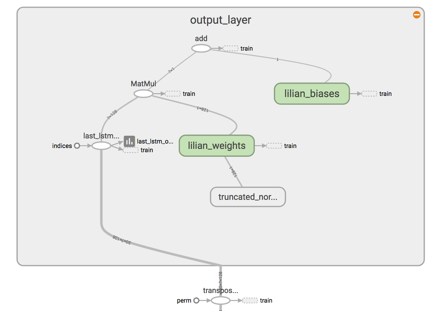
(8) Define weights and biases between the hidden and output layers.

    weight = tf.Variable(tf.truncated_normal([config.lstm_size, config.input_size]))
    bias = tf.Variable(tf.constant(0.1, shape=[config.input_size]))
    prediction = tf.matmul(last, weight) + bias

(9) We use mean square error as the loss metric and the RMSPropOptimizer algorithm for gradient descent optimization.

    loss = tf.reduce_mean(tf.square(prediction - targets))
    optimizer = tf.train.RMSPropOptimizer(learning_rate)
    minimize = optimizer.minimize(loss)

Start Training Session

(1) To start training the graph with real data, we need to start a tf.session first.

with tf.Session(graph=lstm_graph) as sess:

(2) Initialize the variables as defined.

    tf.global_variables_initializer().run()

(0) The learning rates for training epochs should have been precomputed beforehand. The index refers to the epoch index.

learning_rates_to_use = [
    config.init_learning_rate * (
        config.learning_rate_decay ** max(float(i + 1 - config.init_epoch), 0.0)
    ) for i in range(config.max_epoch)]

(3) Each loop below completes one epoch training.

    for epoch_step in range(config.max_epoch):
        current_lr = learning_rates_to_use[epoch_step]
        
        # Check https://github.com/lilianweng/stock-rnn/blob/master/data_wrapper.py
        # if you are curious to know what is StockDataSet and how generate_one_epoch() 
        # is implemented.
        for batch_X, batch_y in stock_dataset.generate_one_epoch(config.batch_size):
            train_data_feed = {
                inputs: batch_X, 
                targets: batch_y, 
                learning_rate: current_lr
            }
            train_loss, _ = sess.run([loss, minimize], train_data_feed)

(4) Don’t forget to save your trained model at the end.

    saver = tf.train.Saver()
    saver.save(sess, "your_awesome_model_path_and_name", global_step=max_epoch_step)

The complete code is available here.

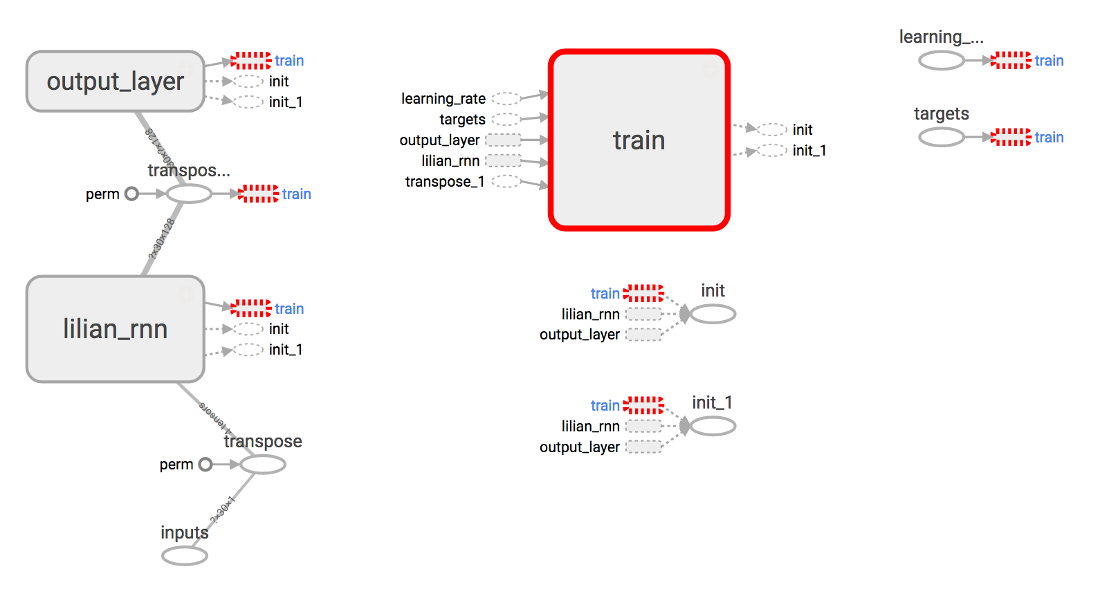
Use TensorBoard

Building the graph without visualization is like drawing in the dark, very obscure and error-prone. Tensorboard provides easy visualization of the graph structure and the learning process. Check out this hand-on tutorial, only 20 min, but it is very practical and showcases several live demos.

Brief Summary

• Use with [tf.name_scope](https://www.tensorflow.org/api_docs/python/tf/name_scope)("your_awesome_module_name"): to wrap elements working on the similar goal together.
• Many tf.* methods accepts name= argument. Assigning a customized name can make your life much easier when reading the graph.
• Methods like tf.summary.scalar and tf.summary.histogram help track the values of variables in the graph during iterations.
• In the training session, define a log file using tf.summary.FileWriter.

with tf.Session(graph=lstm_graph) as sess:
    merged_summary = tf.summary.merge_all()
    writer = tf.summary.FileWriter("location_for_keeping_your_log_files", sess.graph)
    writer.add_graph(sess.graph)

Later, write the training progress and summary results into the file.

_summary = sess.run([merged_summary], test_data_feed)
writer.add_summary(_summary, global_step=epoch_step)  # epoch_step in range(config.max_epoch)

The full working code is available in github.com/lilianweng/stock-rnn.

Results

I used the following configuration in the experiment.

num_layers=1
keep_prob=0.8
batch_size = 64
init_learning_rate = 0.001
learning_rate_decay = 0.99
init_epoch = 5
max_epoch = 100
num_steps=30

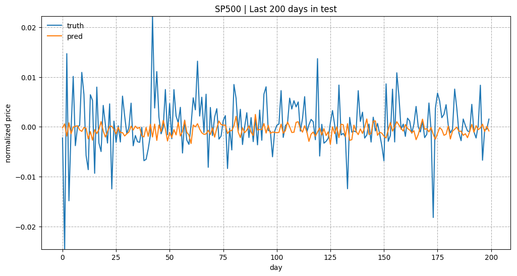
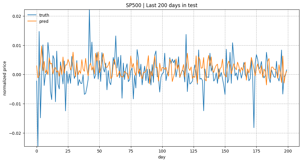
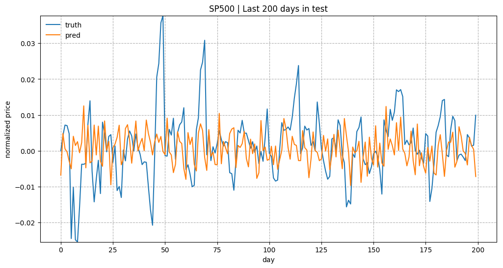
(Thanks to Yury for cathcing a bug that I had in the price normalization. Instead of using the last price of the previous time window, I ended up with using the last price in the same window. The following plots have been corrected.)

Overall predicting the stock prices is not an easy task. Especially after normalization, the price trends look very noisy.

The example code in this tutorial is available in github.com/lilianweng/stock-rnn:scripts.

(Updated on Sep 14, 2017) The model code has been updated to be wrapped into a class: LstmRNN. The model training can be triggered by main.py, such as:

python main.py --stock_symbol=SP500 --train --input_size=1 --lstm_size=128