[Updated on 2022-03-13: add expert choice routing.]
[Updated on 2022-06-10]: Greg and I wrote a shorted and upgraded version of this post, published on OpenAI Blog: “Techniques for Training Large Neural Networks”
In recent years, we are seeing better results on many NLP benchmark tasks with larger pre-trained language models. How to train large and deep neural networks is challenging, as it demands a large amount of GPU memory and a long horizon of training time.
However an individual GPU worker has limited memory and the sizes of many large models have grown beyond a single GPU. There are several parallelism paradigms to enable model training across multiple GPUs, as well as a variety of model architecture and memory saving designs to help make it possible to train very large neural networks.
Training Parallelism
The main bottleneck for training very large neural network models is the intense demand for a large amount of GPU memory, way above what can be hosted on an individual GPU machine. Besides the model weights (e.g. tens of billions of floating point numbers), it is usually even more expensive to store intermediate computation outputs such as gradients and optimizer states (e.g. momentums & variations in Adam). Additionally training a large model often pairs with a large training corpus and thus a single process may just take forever.
As a result, parallelism is necessary. Parallelism can happen at different dimensions, including data, model architecture, and tensor operation.
Data Parallelism
The most naive way for Data parallelism (DP) is to copy the same model weights into multiple workers and assign a fraction of data to each worker to be processed at the same time.
Naive DP cannot work well if the model size is larger than a single GPU node’s memory. Methods like GeePS (Cui et al. 2016) offload temporarily unused parameters back to CPU to work with limited GPU memory when the model is too big to fit into one machine. The data swapping transfer should happen at the backend and not interfere with training computation.
At the end of each minibatch, workers need to synchronize gradients or weights to avoid staleness. There are two main synchronization approaches and both have clear pros & cons.
- Bulk synchronous parallels (BSP): Workers sync data at the end of every minibatch. It prevents model weights staleness and good learning efficiency but each machine has to halt and wait for others to send gradients.
- Asynchronous parallel (ASP): Every GPU worker processes the data asynchronously, no waiting or stalling. However, it can easily lead to stale weights being used and thus lower the statistical learning efficiency. Even though it increases the computation time, it may not speed up training time to convergence.
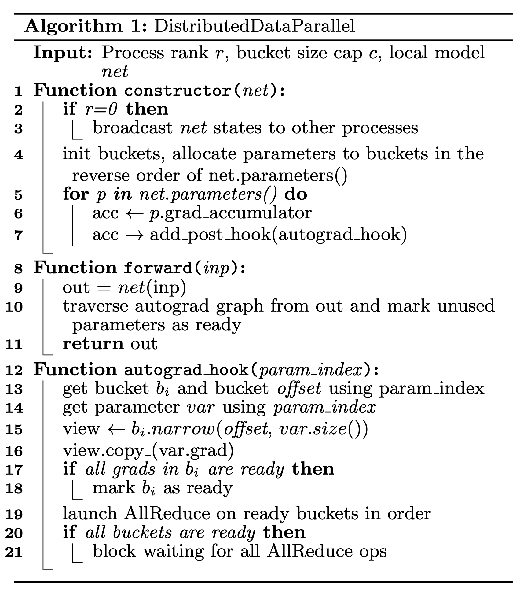
Somewhere in the middle is to synchronize gradients globally once every $x$ iterations ($x > 1$). This feature is called “gradient accumulation” in Distribution Data Parallel (DDP) since Pytorch v1.5 (Li et al. 2021). Bucketing gradients avoid immediate AllReduce operations but instead buckets multiple gradients into one AllReduce to improve throughput. Computation and communication scheduling optimization can be made based on the computation graph.
Model Parallelism
Model parallelism (MP) aims to solve the case when the model weights cannot fit into a single node. The computation and model parameters are partitioned across multiple machines. Different from data parallelism where each worker hosts a full copy of the entire model, MP only allocates a fraction of model parameters on one worker and thus both the memory usage and the computation are reduced.
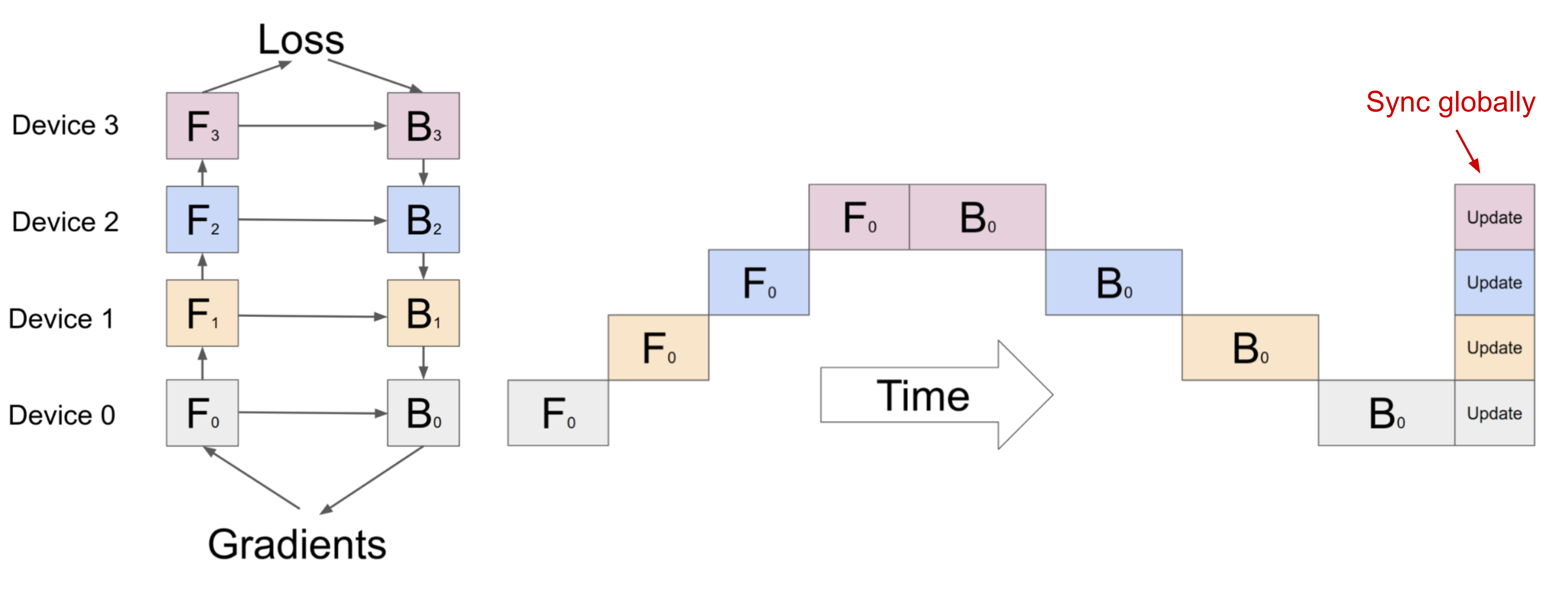
Since deep neural networks usually contain a stack of vertical layers, it feels straightforward to split a large model by layer, where a small consecutive set of layers are grouped into one partition on one worker. However, a naive implementation for running every data batch through multiple such workers with sequential dependency leads to big bubbles of waiting time and severe under-utilization of computation resources.
Pipeline Parallelism
Pipeline parallelism (PP) combines model parallelism with data parallelism to reduce inefficient time “bubbles’’. The main idea is to split one minibatch into multiple microbatches and enable each stage worker to process one microbatch simultaneously. Note that every microbatch needs two passes, one forward and one backward. Inter-worker communication only transfers activations (forward) and gradients (backward). How these passes are scheduled and how the gradients are aggregated vary in different approaches. The number of partitions (workers) is also known as pipeline depth.
In GPipe (Huang et al. 2019) gradients from multiple microbatches are aggregated and applied synchronously at the end. The synchronous gradient descent guarantees learning consistency and efficiency irrespective of the number of workers. As shown in Fig. 3, bubbles still exist but are much smaller than what’s in Given $m$ evenly split microbatches and $d$ partitions, assuming both forward and backward per microbatch take one unit of time, the fraction of bubble is:
The GPipe paper observed that the bubble overhead is almost negligible if the number of microbatches is more than 4x the number of partitions $m > 4d$ (when activation recomputation is applied).
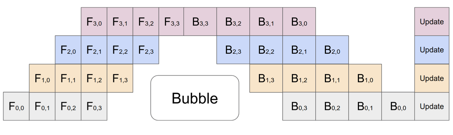
GPipe achieves almost linear speedup in throughput with the number of devices, although it is not always guaranteed if the model parameters are not evenly distributed across workers.
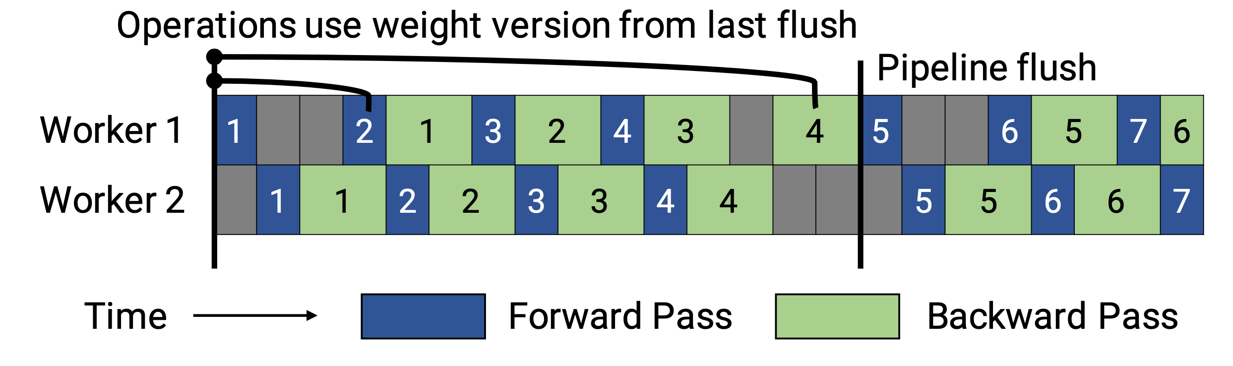
PipeDream (Narayanan et al. 2019) schedules each worker to alternatively process the forward and backward passes (1F1B).
PipeDream names each model partition “stage” and each stage worker can have multiple replicas to run data parallelism. In this process, PipeDream uses a deterministic round-robin load balancing strategy to assign work among multiple replicas of stages to ensure that the forward and backward passes for the same minibatch happen on the same replica.
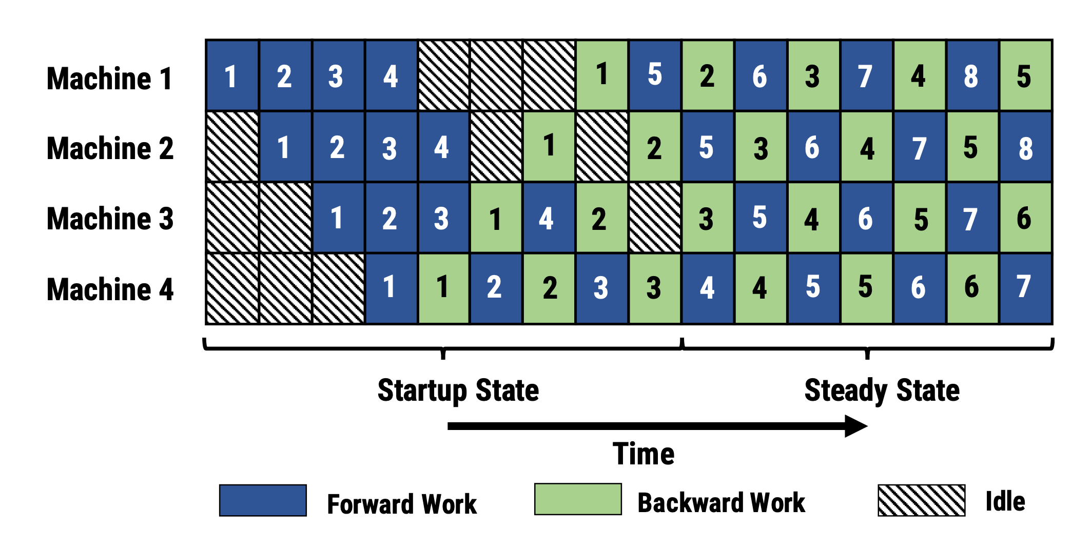
Since PipeDream does not have an end-of-batch global gradient sync across all the workers, an native implementation of 1F1B can easily lead to the forward and backward passes of one microbatch using different versions of model weights, thus lowering the learning efficiency. PipeDream proposed a few designs to tackle this issue:
- Weight stashing: Each worker keeps track of several model versions and makes sure that the same version of weights are used in the forward and backward passes given one data batch.
- Vertical sync (Optional): The version of model weights flows between stage workers together with activations and gradients. Then the computation adopts the corresponding stashed version propagated from the previous worker. This process keeps version consistency across workers. Note that it is asynchronous, different from GPipe.
At the beginning of a training run, PipeDream first profiles the computation memory cost and time of each layer in the model and then optimizes a solution for partitioning layers into stages, which is a dynamic programming problem.
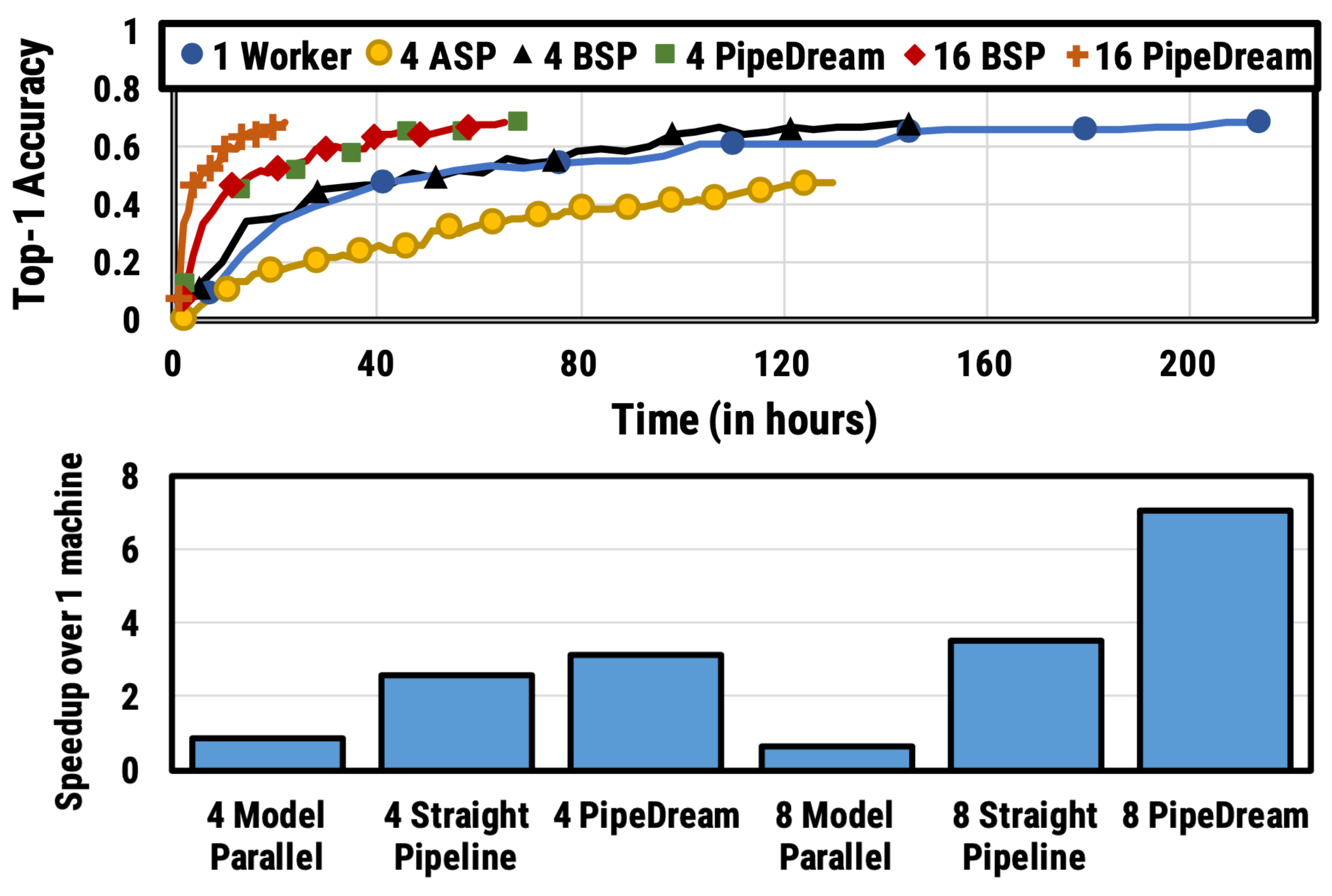
Two variations of PipeDream were later proposed to reduce the memory footprint by stashed model versions (Narayanan et al. 2021).
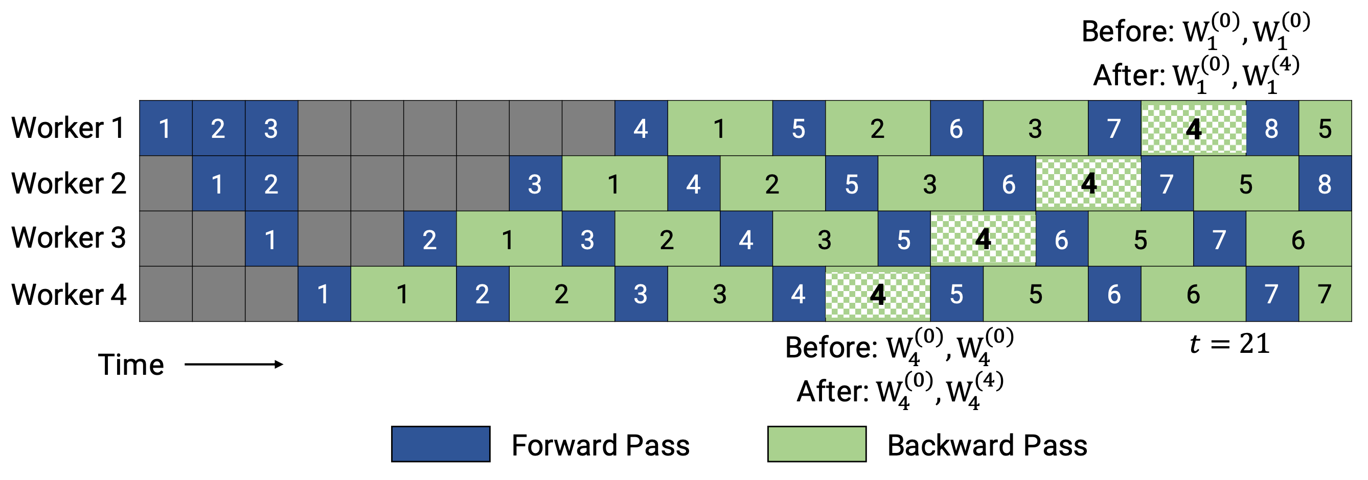
PipeDream-flush adds a globally synchronized pipeline flush periodically, just like GPipe. In this way, it greatly reduces the memory footprint (i.e. only maintain a single version of model weights) by sacrificing a little throughput.
PipeDream-2BW maintains only two versions of model weights, where “2BW” is short for “double-buffered weights”. It generates a new model version every $k$ microbatches and $k$ should be larger than the pipeline depth $d$, $k > d$. A newly updated model version cannot fully replace the old version immediately since some leftover backward passes still depend on the old version. In total only two versions need to be saved so the memory cost is much reduced.
Tensor Parallelism
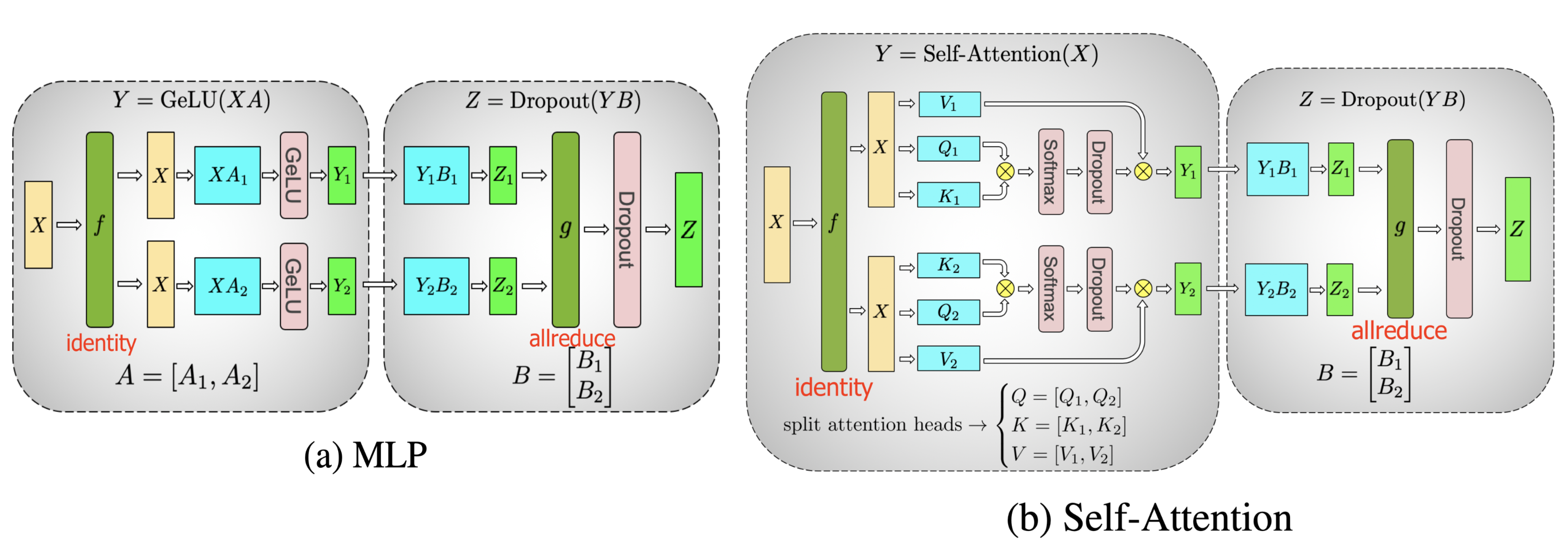
Both model and pipeline parallelisms split a model vertically. OTOH we can horizontally partition the computation for one tensor operation across multiple devices, named Tensor parallelism (TP).
Let’s take the transformer as an example given its popularity. The transformer model mainly consists of layers of MLP and self-attention blocks. Megatron-LM (Shoeybi et al. 2020) adopts a simple way to parallelize intra-layer computation for MLP and self-attention.
A MLP layer in a transformer contains a GEMM (General matrix multiply) followed by an non-linear GeLU transfer. Let’s split weight matrix $A$ by column:
The attention block runs GEMM with query ($Q$), key ($K$), and value weights ($V$) according to the above partitioning in parallel and then combines them with another GEMM to produce the attention head results.
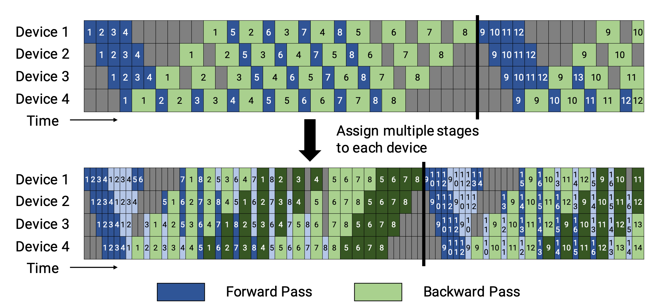
Narayanan et al. (2021) combined pipeline, tensor and data parallelism with a new pipeline scheduling strategy and named their approach PTD-P. Instead of only positioning a continuous set of layers (“model chunk”) on a device, each worker can be assigned with multiple chunks of smaller continuous subsets of layers (e.g. device 1 has layers 1, 2, 9, 10; device 2 has layers 3, 4, 11, 12; each has two model chunks). The number of microbatches in one batch should be exactly divided by the number of workers ($m % d = 0$). If there are $v$ model chunks per worker, the pipeline bubble time can be reduced by a multiplier of $v$ compared to a GPipe scheduling.
Mixture-of-Experts (MoE)
The Mixture-of-Experts (MoE) approach attracts a lot of attention recently as researchers (mainly from Google) try to push the limit of model size. The core of the idea is ensembling learning: Combination of multiple weak learners gives you a strong learner!
Within one deep neural network, ensembling can be implemented with a gating mechanism connecting multiple experts (Shazeer et al., 2017). The gating mechanism controls which subset of the network (e.g. which experts) should be activated to produce outputs. The paper named it “sparsely gated mixture-of-experts” (MoE) layer.
Precisely one MoE layer contains
- $n$ feed-forward networks as experts $\{E_i\}^n_{i=1}$
- A trainable gating network $G$ to learn a probability distribution over $n$ experts so as to route the traffic to a few selected experts.
Depending on the gating outputs, not every expert has to be evaluated. When the number of experts is too large, we can consider using a two-level hierarchical MoE.
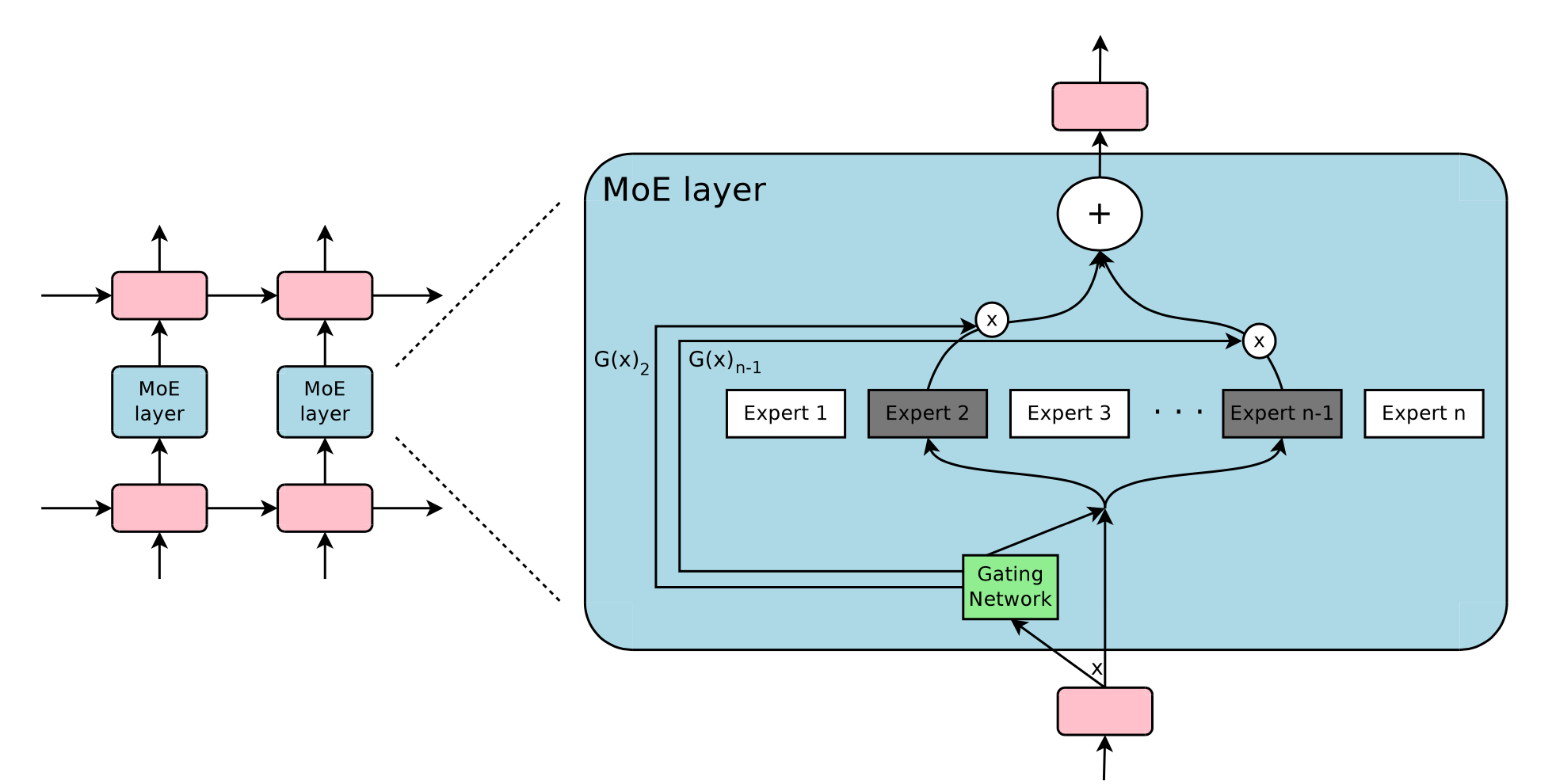
A simple choice of $G$ is to multiply the input with a trainable weight matrix $G_g$ and then do softmax: $G_\sigma (x) = \text{softmax}(x W_g)$. However, this produces a dense control vector for gating and does not help save computation resources because we don’t need to evaluate an expert only when $G^{(i)}(x)=0$. Thus the MoE layer only keeps the top $k$ values. It also adds tunable Gaussian noise into $G$ to improve load balancing. This mechanism is called noisy top-k gating.
where the superscript $v^{(i)}$ denotes the i-th dimension of the vector $v$. The function $\text{topk}(., k)$ selected the top $k$ dimensions with highest values by setting other dimensions to $-\infty$.
To avoid the self-reinforcing effect that the gating network may favor a few strong experts all the time, Shazeer et al. (2017) proposed a soft constraint via an additional importance loss to encourage all the experts to have the same weights. It is equivalent to the square of the coefficient of variation of batchwise average value per expert.
where $ \text{CV}$ is the coefficient of variation and the loss weight $w_\text{aux}$ is a hyperparameter to tune.
Because every expert network only gets a fraction of training samples (“The shrinking batch problem”), we should try to use a batch size as large as possible in MoE. However, it is restricted by GPU memory. Data parallelism and model parallelism can be applied to improve the throughput.
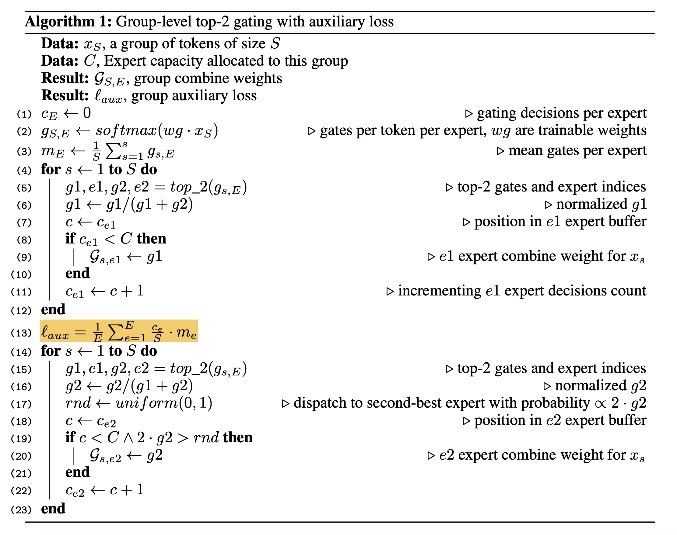
GShard (Lepikhin et al., 2020) scales the MoE transformer model up to 600 billion parameters with sharding. The MoE transformer replaces every other feed forward layer with a MoE layer. The sharded MoE transformer only has the MoE layers sharded across multiple machines, while other layers are simply duplicated.
There are several improved designs for the gating function $G$ in GShard:
- Expert capacity: The amount of tokens going through one expert should not go above a threshold, named “expert capacity”. If a token is routed to experts that have reached their capacity, the token would be marked “overflowed” and the gating output is changed to a zero vector.
- Local group dispatching: Tokens are evenly partitioned into multiple local groups and the expert capacity is enforced on the group level.
- Auxiliary loss: The motivation is similar to the original MoE aux loss. They add an auxiliary loss to minimize the mean square of the fraction of data routed to each expert.
- Random routing: The 2nd-best expert is selected with a probability proportional to its weight; otherwise, GShard follows a random routing, so as to add some randomness.
Switch Transformer (Fedus et al. 2021) scales the model size up to trillions of parameters (!!) by replacing the dense feed forward layer with a sparse switch FFN layer in which each input is only routed to one expert network. The auxiliary loss for load balancing is $\text{loss}_\text{aux} = w_\text{aux} \sum_{i=1}^n f_i p_i$ given $n$ experts, where $f_i$ is the fraction of tokens routed to the $i$-th expert and $p_i$ is the routing probability for expert $i$ predicted by the gating network.
To improve training stability, switch transformer incorporates the following designs:
- Selective precision. They showed that selectively casting only a local part of the model to FP32 precision improves stability, while avoiding the expensive communication cost of FP32 tensors. The FP32 precision is only used within the body of the router function and the results are recast to FP16.
- Smaller initialization. The initialization of weight matrices is sampled from a truncated normal distribution with mean $\mu=0$ and stdev $\sigma = \sqrt{s/n}$. They also recommended reducing the transformer initialization scale parameter $s=1$ to $s=0.1$.
- Use higher expert dropout. Fine-tuning often works with a small dataset. To avoid overfitting, the dropout rate within each expert is increased by a significant amount. Interestingly they found that increasing dropout across all layers lead to poor performance. In the paper, they used a dropout rate 0.1 at non-expert layers but 0.4 within expert FF layers.
The switch transformer paper summarized different data and model parallelism strategies for training large models with a nice illustration:
Both GShard top-2 and Switch Transformer top-1 depend on token choice, where each token picks the best one or two experts to route through. They both adopt an auxiliary loss to encourage more balanced load allocation but it does not guarantee the best performance. Furthermore, the expert capacity limit may lead to wasted tokens as they would be discarded if an expert reaches its capacity limit.
Export Choice (EC) (Zhou et al. 2022) routing instead enables each expert to select the top-$k$ tokens. In this way, each expert naturally guarantees a fixed capacity and each token may be routed to multiple experts. EC can achieve perfect load balancing and is shown to improve training convergence by 2x.
Given $e$ experts and an input matrix $X \in \mathbb{R}^{n \times d}$, the token-to-expert affinity scores are computed by: $$ S = \text{softmax}(X \cdot W_g), \text{where } W_g \in \mathbb{R}^{d \times e}, S \in \mathbb{R}^{n \times e} $$
A token-to-expert assignment is represented by three matrices, $I, G \in \mathbb{R}^{e\times k}$ and $P \in \mathbb{R}^{e \times k \times n}$. $I[i,j]$ annotates which token is the $j$-th selection by the $i$-th expert. The gating matrix $G$ stores the routing weights of selected tokens. $P$ is the one-hot version of $I$, used to produce the input matrix ($P \cdot X \in \mathbb{R}^{e \times k \times d}$) for the gated FFN layer. $$ G, I = \text{top-k}(S^\top, k)\quad P = \text{one-hot}(I) $$
One regularization that export choice routing explored is to limit the maximum number of experts per token.
where each entry $A[i,j]$ in $A \in \mathbb{R}^{e \times n}$ marks whether the $i$-the expert selects the $j$-th token. Solving this is non-trivial. The paper used Dykstra’s algorithm that runs a sequence of multiple iterative computation steps. Capped expert choice results in a slight decrease in the fine-tuning performance in the experiments.
The parameter $k$ is determined by $k=nc/e$, where $n$ is the total number of tokens in one batch and $c$ is a capacity factor indicating the average number of experts used by one token. The paper used $c=2$ in most experiments, but EC with $c=1$ still outperforms the top-1 token choice gating. Interestingly, $c=0.5$ only marginally hurts the training performance.
One big drawback of EC is that it does not work when the batch size is too small, neither for auto-regressive text generation, because it needs to know the future tokens to do the top-$k$ selection.
Other Memory Saving Designs
CPU Offloading
When the GPU memory is full, one option is to offload temporarily unused data to CPU and read them back when needed later (Rhu et al. 2016). The idea of CPU offloading is straightforward but is less popular in recent years due to the slowdown it brings into the training time.
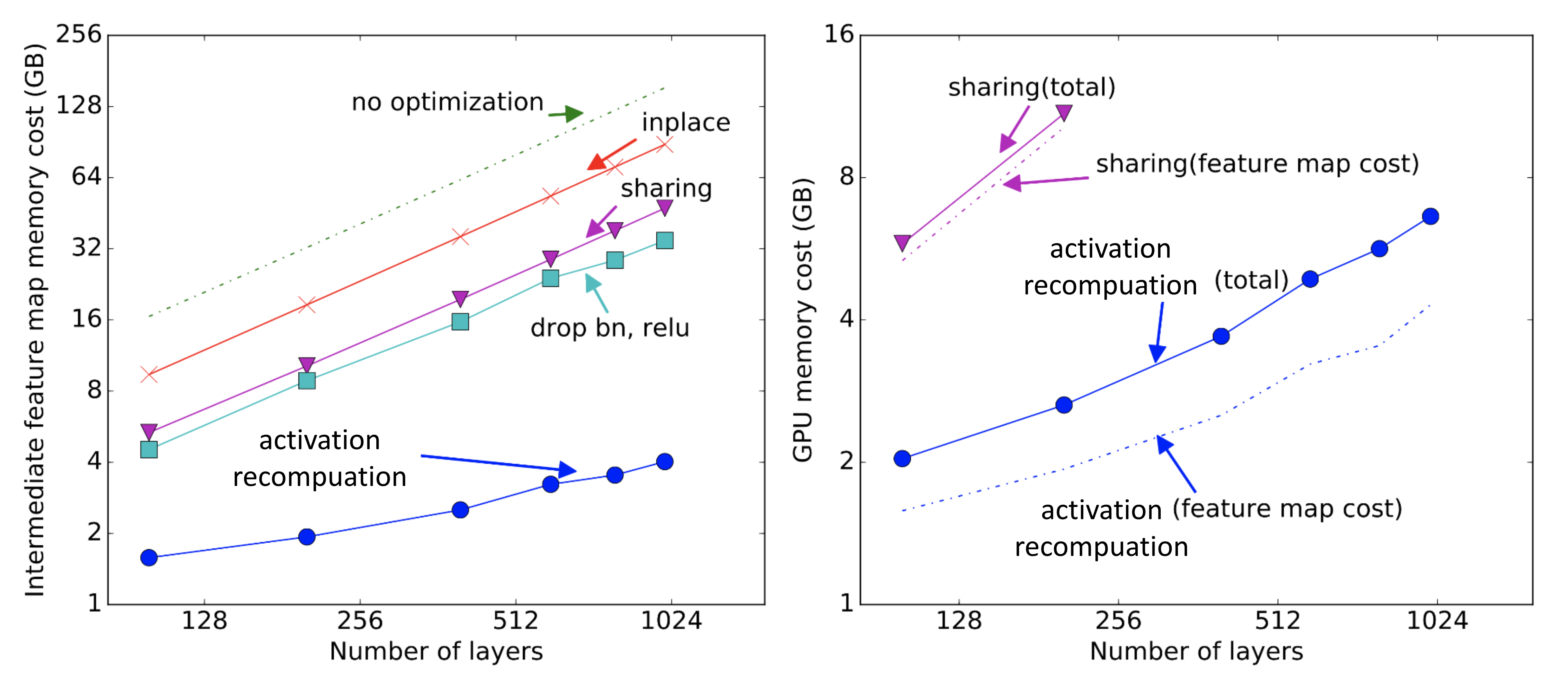
Activation Recomputation
Activation recomputation (also known as “activation checkpointing” or “gradient checkpointing”; Chen et al. 2016) is a smart yet simple idea to reduce memory footprint at the cost of computation time. It reduces the memory cost of training a $\ell$ layer deep neural net to $O(\sqrt{\ell})$, which only additionally consumes an extra forward pass computation per batch.
Let’s say, we evenly divide an $\ell$-layer network into $d$ partitions. Only activations at partition boundaries are saved and communicated between workers. Intermediate activations at intra-partition layers are still needed for computing gradients so they are recomputed during backward passes. With activation recomputation, the memory cost for training $M(\ell)$ is:
The minimum cost is $O(\sqrt{\ell})$ at $d=\sqrt{\ell}$.
Activation recompuation trick can give sublinear memory cost with respect to the model size.
Mixed Precision Training
Narang & Micikevicius et al. (2018) introduced a method to train models using half-precision floating point (FP16) numbers without losing model accuracy.
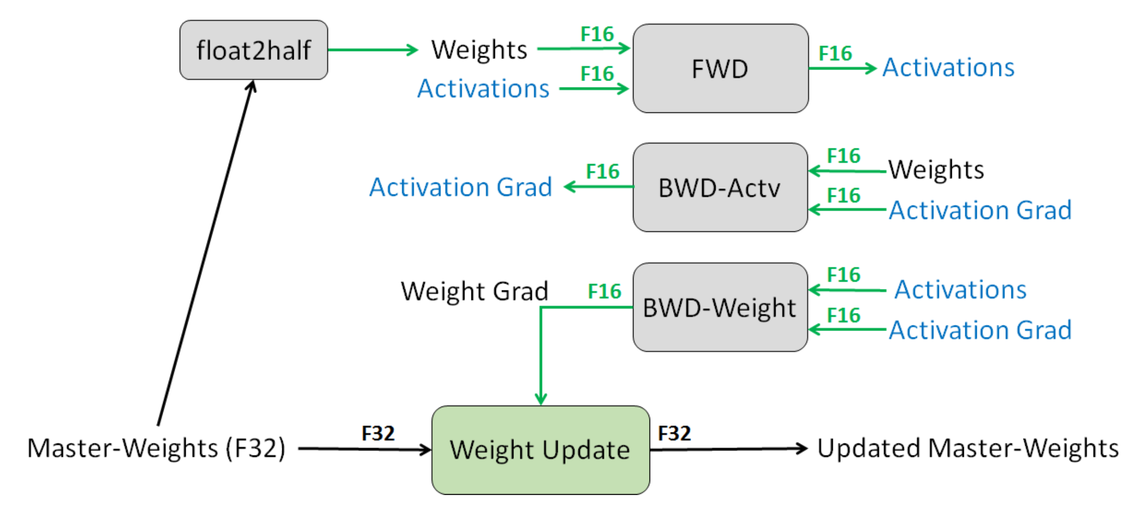
Three techniques to avoid losing critical information at half-precision:
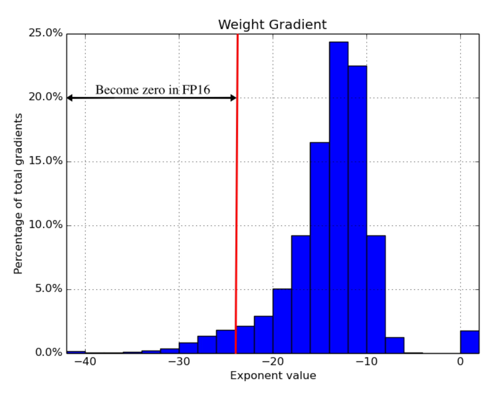
- Full-precision master copy of weights. Maintain a full precision (FP32) copy of model weights that accumulates gradients. The numbers are rounded up to half-precision for forward & backward passes. The motivation is that each gradient update (i.e. gradient times the learning rate) might be too small to be fully contained within the FP16 range (i.e. $2^{-24}$ becomes zero in FP16).
- Loss scaling. Scale up the loss to better handle gradients with small magnitudes (See Fig. 16). Scaling up the gradients helps shift them to occupy a larger section towards the right section (containing larger values) of the representable range, preserving values that are otherwise lost.
- Arithmetic precision. For common network arithmetic (e.g. vector dot-product, reduction by summing up vector elements), we can accumulate the partial results in FP32 and then save the final output as FP16 before saving into memory. Point-wise operations can be executed in either FP16 or FP32.
In their experiments, loss scaling is not needed for some networks (e.g. image classification, Faster R-CNN), but necessary for others (e.g. Multibox SSD, big LSTM language model).
Compression
Intermediate results often consume a lot of memory, although they are only needed in one forward pass and one backward pass. There is a noticeable temporal gap between these two uses. Thus Jain et al. (2018) proposed a data encoding strategy to compress the intermediate results after the first use in the first pass and then decode it back for back-propagation later.
Their system Gist incorporates two encoding schemes: Layer-specific lossless encoding; focus on ReLU-Pool (“Binarize”) and ReLU-Conv (“Sparse storage and dense computation”) patterns. Aggressive lossy encoding; use delayed precision reduction (DPR). They observed that the first immediate use of feature maps should be kept at high precision but the second use can tolerate lower precision.
The experiments showed that Gist can reduce the memory cost by 2x across 5 SOTA image classification DNNs, with an average of 1.8x with only 4% performance overhead.
Memory Efficient Optimizer
Optimizers are eager for memory consumption. Take the popular Adam optimizer as an example, it internally needs to maintain momentums and variances, both at the same scale as gradients and model parameters. All out of a sudden, we need to save 4x the memory of model weights.
Several optimizers have been proposed to reduce the memory footprint. For example, instead of storing the full momentums and variations as in Adam, Adafactor (Shazeer et al. 2018) only tracks the per-row and per-column sums of the moving averages and then estimates the second moments based on these sums. SM3 (Anil et al. 2019) describes a different adaptive optimization method, leading to largely reduced memory as well.
ZeRO (Zero Redundancy Optimizer; Rajbhandari et al. 2019) optimizes the memory used for training large models based on the observation about two major memory consumption of large model training:
- The majority is occupied by model states, including optimizer states (e.g. Adam momentums and variances), gradients and parameters. Mixed-precision training demands a lot of memory since the optimizer needs to keep a copy of FP32 parameters and other optimizer states, besides the FP16 version.
- The remaining is consumed by activations, temporary buffers and unusable fragmented memory (named residual states in the paper).
ZeRO combines two approaches, ZeRO-DP and ZeRO-R. ZeRO-DP is an enhanced data parallelism to avoid simple redundancy over model states. It partitions optimizer state, gradients and parameters across multiple data parallel processes via a dynamic communication schedule to minimize the communication volume. ZeRO-R optimizes the memory consumption of residual states, using partitioned activation recomputation, constant buffer size and on-the-fly memory defragmentation.
Citation
Cited as:
Weng, Lilian. (Sep 2021). How to train really large models on many GPUs? Lil’Log. https://lilianweng.github.io/posts/2021-09-25-train-large/.
Or
@article{weng2021large,
  title   = "How to Train Really Large Models on Many GPUs?",
  author  = "Weng, Lilian",
  journal = "lilianweng.github.io",
  year    = "2021",
  month   = "Sep",
  url     = "https://lilianweng.github.io/posts/2021-09-25-train-large/"
}
References
[1] Li et al. “PyTorch Distributed: Experiences on Accelerating Data Parallel Training” VLDB 2020.
[2] Cui et al. “GeePS: Scalable deep learning on distributed GPUs with a GPU-specialized parameter server” EuroSys 2016
[3] Shoeybi et al. “Megatron-LM: Training Multi-Billion Parameter Language Models Using Model Parallelism.” arXiv preprint arXiv:1909.08053 (2019).
[4] Narayanan et al. “Efficient Large-Scale Language Model Training on GPU Clusters Using Megatron-LM.” arXiv preprint arXiv:2104.04473 (2021).
[5] Huang et al. “GPipe: Efficient Training of Giant Neural Networks using Pipeline Parallelism.” arXiv preprint arXiv:1811.06965 (2018).
[6] Narayanan et al. “PipeDream: Generalized Pipeline Parallelism for DNN Training.” SOSP 2019.
[7] Narayanan et al. “Memory-Efficient Pipeline-Parallel DNN Training.” ICML 2021.
[8] Shazeer et al. “The Sparsely-Gated Mixture-of-Experts Layer Noam.” arXiv preprint arXiv:1701.06538 (2017).
[9] Lepikhin et al. “GShard: Scaling Giant Models with Conditional Computation and Automatic Sharding.” arXiv preprint arXiv:2006.16668 (2020).
[10] Fedus et al. “Switch Transformers: Scaling to Trillion Parameter Models with Simple and Efficient Sparsity.” arXiv preprint arXiv:2101.03961 (2021).
[11] Narang & Micikevicius, et al. “Mixed precision training.” ICLR 2018.
[12] Chen et al. 2016 “Training Deep Nets with Sublinear Memory Cost.” arXiv preprint arXiv:1604.06174 (2016).
[13] Jain et al. “Gist: Efficient data encoding for deep neural network training.” ISCA 2018.
[14] Shazeer & Stern. “Adafactor: Adaptive learning rates with sublinear memory cost.” arXiv preprint arXiv:1804.04235 (2018).
[15] Anil et al. “Memory-Efficient Adaptive Optimization.” arXiv preprint arXiv:1901.11150 (2019).
[16] Rajbhandari et al. “ZeRO: Memory Optimization Towards Training A Trillion Parameter Models Samyam.” arXiv preprint arXiv:1910.02054 (2019).
[17] Zhou et al. “Mixture-of-Experts with Expert Choice Routing” arXiv preprint arXiv:2202.09368 (2022).