[Updated on 2020-06-17: Add “exploration via disagreement” in the “Forward Dynamics” section.

Exploitation versus exploration is a critical topic in Reinforcement Learning. We’d like the RL agent to find the best solution as fast as possible. However, in the meantime, committing to solutions too quickly without enough exploration sounds pretty bad, as it could lead to local minima or total failure. Modern RL algorithms that optimize for the best returns can achieve good exploitation quite efficiently, while exploration remains more like an open topic.

I would like to discuss several common exploration strategies in Deep RL here. As this is a very big topic, my post by no means can cover all the important subtopics. I plan to update it periodically and keep further enriching the content gradually in time.

Classic Exploration Strategies

As a quick recap, let’s first go through several classic exploration algorithms that work out pretty well in the multi-armed bandit problem or simple tabular RL.

• Epsilon-greedy: The agent does random exploration occasionally with probability $\epsilon$ and takes the optimal action most of the time with probability $1-\epsilon$.
• Upper confidence bounds: The agent selects the greediest action to maximize the upper confidence bound $\hat{Q}_t(a) + \hat{U}_t(a)$, where $\hat{Q}_t(a)$ is the average rewards associated with action $a$ up to time $t$ and $\hat{U}_t(a)$ is a function reversely proportional to how many times action $a$ has been taken. See here for more details.
• Boltzmann exploration: The agent draws actions from a boltzmann distribution (softmax) over the learned Q values, regulated by a temperature parameter $\tau$.
• Thompson sampling: The agent keeps track of a belief over the probability of optimal actions and samples from this distribution. See here for more details.

The following strategies could be used for better exploration in deep RL training when neural networks are used for function approximation:

• Entropy loss term: Add an entropy term $H(\pi(a \vert s))$ into the loss function, encouraging the policy to take diverse actions.
• Noise-based Exploration: Add noise into the observation, action or even parameter space (Fortunato, et al. 2017, Plappert, et al. 2017).

Key Exploration Problems

Good exploration becomes especially hard when the environment rarely provides rewards as feedback or the environment has distracting noise. Many exploration strategies are proposed to solve one or both of the following problems.

The Hard-Exploration Problem

The “hard-exploration” problem refers to exploration in an environment with very sparse or even deceptive reward. It is difficult because random exploration in such scenarios can rarely discover successful states or obtain meaningful feedback.

Montezuma’s Revenge is a concrete example for the hard-exploration problem. It remains as a few challenging games in Atari for DRL to solve. Many papers use Montezuma’s Revenge to benchmark their results.

The Noisy-TV Problem

The “Noisy-TV” problem started as a thought experiment in Burda, et al (2018). Imagine that an RL agent is rewarded with seeking novel experience, a TV with uncontrollable & unpredictable random noise outputs would be able to attract the agent’s attention forever. The agent obtains new rewards from noisy TV consistently, but it fails to make any meaningful progress and becomes a “couch potato”.

Intrinsic Rewards as Exploration Bonuses

One common approach to better exploration, especially for solving the hard-exploration problem, is to augment the environment reward with an additional bonus signal to encourage extra exploration. The policy is thus trained with a reward composed of two terms, $r_t = r^e_t + \beta r^i_t$, where $\beta$ is a hyperparameter adjusting the balance between exploitation and exploration.

• $r^e_t$ is an extrinsic reward from the environment at time $t$, defined according to the task in hand.
• $r^i_t$ is an intrinsic exploration bonus at time $t$.

This intrinsic reward is somewhat inspired by intrinsic motivation in psychology (Oudeyer & Kaplan, 2008). Exploration driven by curiosity might be an important way for children to grow and learn. In other words, exploratory activities should be rewarding intrinsically in the human mind to encourage such behavior. The intrinsic rewards could be correlated with curiosity, surprise, familiarity of the state, and many other factors.

Same ideas can be applied to RL algorithms. In the following sections, methods of bonus-based exploration rewards are roughly grouped into two categories:

1. Discovery of novel states
2. Improvement of the agent’s knowledge about the environment.

Count-based Exploration

If we consider intrinsic rewards as rewarding conditions that surprise us, we need a way to measure whether a state is novel or appears often. One intuitive way is to count how many times a state has been encountered and to assign a bonus accordingly. The bonus guides the agent’s behavior to prefer rarely visited states to common states. This is known as the count-based exploration method.

Let $N_n(s)$ be the empirical count function that tracks the real number of visits of a state $s$ in the sequence of $s_{1:n}$. Unfortunately, using $N_n(s)$ for exploration directly is not practical, because most of the states would have $N_n(s)=0$, especially considering that the state space is often continuous or high-dimensional. We need an non-zero count for most states, even when they haven’t been seen before.

Counting by Density Model

Bellemare, et al. (2016) used a density model to approximate the frequency of state visits and a novel algorithm for deriving a pseudo-count from this density model. Let’s first define a conditional probability over the state space, $\rho_n(s) = \rho(s \vert s_{1:n})$ as the probability of the $(n+1)$-th state being $s$ given the first $n$ states are $s_{1:n}$. To measure this empirically, we can simply use $N_n(s)/n$.

Let’s also define a recoding probability of a state $s$ as the probability assigned by the density model to $s$ after observing a new occurrence of $s$, $\rho’_n(s) = \rho(s \vert s_{1:n}s)$.

The paper introduced two concepts to better regulate the density model, a pseudo-count function $\hat{N}_n(s)$ and a pseudo-count total $\hat{n}$. As they are designed to imitate an empirical count function, we would have:

The relationship between $\rho_n(x)$ and $\rho’_n(x)$ requires the density model to be learning-positive: for all $s_{1:n} \in \mathcal{S}^n$ and all $s \in \mathcal{S}$, $\rho_n(s) \leq \rho’_n(s)$. In other words, After observing one instance of $s$, the density model’s prediction of that same $s$ should increase. Apart from being learning-positive, the density model should be trained completely online with non-randomized mini-batches of experienced states, so naturally we have $\rho’_n = \rho_{n+1}$.

The pseudo-count can be computed from $\rho_n(s)$ and $\rho’_n(s)$ after solving the above linear system:

Or estimated by the prediction gain (PG):

A common choice of a count-based intrinsic bonus is $r^i_t = N(s_t, a_t)^{-1/2}$ (as in MBIE-EB; Strehl & Littman, 2008). The pseudo-count-based exploration bonus is shaped in a similar form, $r^i_t = \big(\hat{N}_n(s_t, a_t) + 0.01 \big)^{-1/2}$.

Experiments in Bellemare et al., (2016) adopted a simple CTS (Context Tree Switching) density model to estimate pseudo-counts. The CTS model takes as input a 2D image and assigns to it a probability according to the product of location-dependent L-shaped filters, where the prediction of each filter is given by a CTS algorithm trained on past images. The CTS model is simple but limited in expressiveness, scalability, and data efficiency. In a following-up paper, Georg Ostrovski, et al. (2017) improved the approach by training a PixelCNN (van den Oord et al., 2016) as the density model.

The density model can also be a Gaussian Mixture Model as in Zhao & Tresp (2018). They used a variational GMM to estimate the density of trajectories (e.g. concatenation of a sequence of states) and its predicted probabilities to guide prioritization in experience replay in off-policy setting.

Counting after Hashing

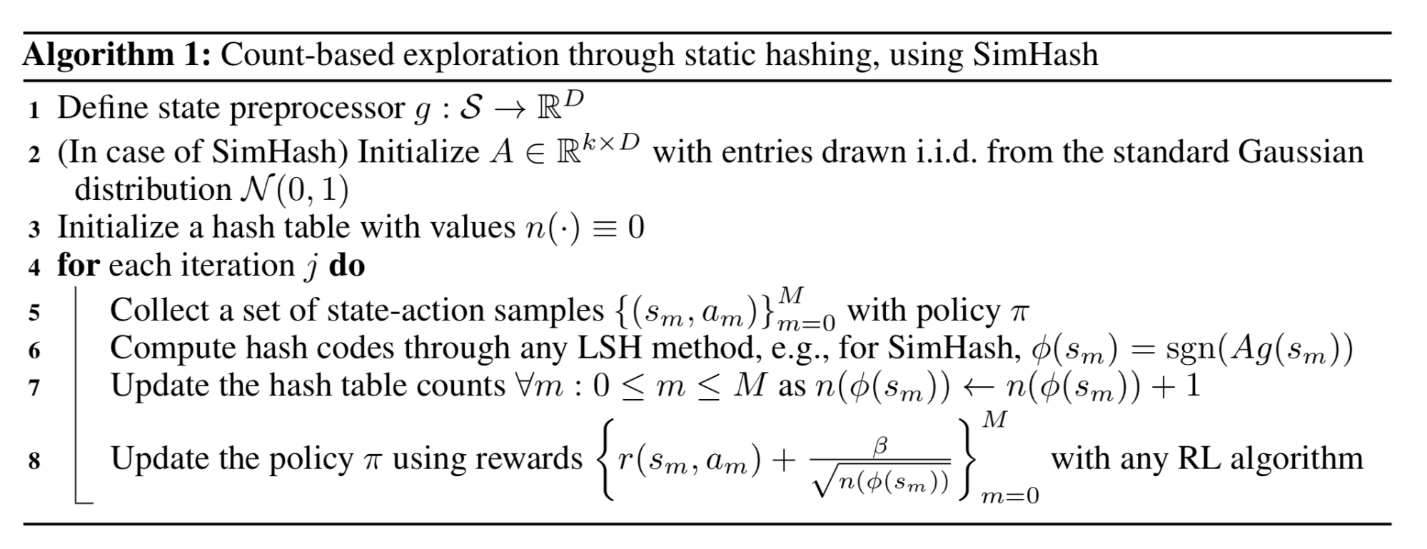
Another idea to make it possible to count high-dimensional states is to map states into hash codes so that the occurrences of states become trackable (Tang et al. 2017). The state space is discretized with a hash function $\phi: \mathcal{S} \mapsto \mathbb{Z}^k$. An exploration bonus $r^{i}: \mathcal{S} \mapsto \mathbb{R}$ is added to the reward function, defined as $r^{i}(s) = {N(\phi(s))}^{-1/2}$, where $N(\phi(s))$ is an empirical count of occurrences of $\phi(s)$.

Tang et al. (2017) proposed to use Locality-Sensitive Hashing (LSH) to convert continuous, high-dimensional data to discrete hash codes. LSH is a popular class of hash functions for querying nearest neighbors based on certain similarity metrics. A hashing scheme $x \mapsto h(x)$ is locality-sensitive if it preserves the distancing information between data points, such that close vectors obtain similar hashes while distant vectors have very different ones. (See how LSH is used in Transformer improvement if interested.) SimHash is a type of computationally efficient LSH and it measures similarity by angular distance:

where $A \in \mathbb{R}^{k \times D}$ is a matrix with each entry drawn i.i.d. from a standard Gaussian and $g: \mathcal{S} \mapsto \mathbb{R}^D$ is an optional preprocessing function. The dimension of binary codes is $k$, controlling the granularity of the state space discretization. A higher $k$ leads to higher granularity and fewer collisions.

For high-dimensional images, SimHash may not work well on the raw pixel level. Tang et al. (2017) designed an autoencoder (AE) which takes as input states $s$ to learn hash codes. It has one special dense layer composed of $k$ sigmoid functions as the latent state in the middle and then the sigmoid activation values $b(s)$ of this layer are binarized by rounding to their closest binary numbers $\lfloor b(s)\rceil \in \{0, 1\}^D$ as the binary hash codes for state $s$. The AE loss over $n$ states includes two terms:

One problem with this approach is that dissimilar inputs $s_i, s_j$ may be mapped to identical hash codes but the AE still reconstructs them perfectly. One can imagine replacing the bottleneck layer $b(s)$ with the hash codes $\lfloor b(s)\rceil$, but then gradients cannot be back-propagated through the rounding function. Injecting uniform noise could mitigate this effect, as the AE has to learn to push the latent variable far apart to counteract the noise.

Prediction-based Exploration

The second category of intrinsic exploration bonuses are rewarded for improvement of the agent’s knowledge about the environment. The agent’s familiarity with the environment dynamics can be estimated through a prediction model. This idea of using a prediction model to measure curiosity was actually proposed quite a long time ago (Schmidhuber, 1991).

Forward Dynamics

Learning a forward dynamics prediction model is a great way to approximate how much knowledge our model has obtained about the environment and the task MDPs. It captures an agent’s capability of predicting the consequence of its own behavior, $f: (s_t, a_t) \mapsto s_{t+1}$. Such a model cannot be perfect (e.g. due to partial observation), the error $e(s_t, a_t) = | f(s_t, a_t) - s_{t+1} |^2_2$ can be used for providing intrinsic exploration rewards. The higher the prediction error, the less familiar we are with that state. The faster the error rate drops, the more learning progress signals we acquire.

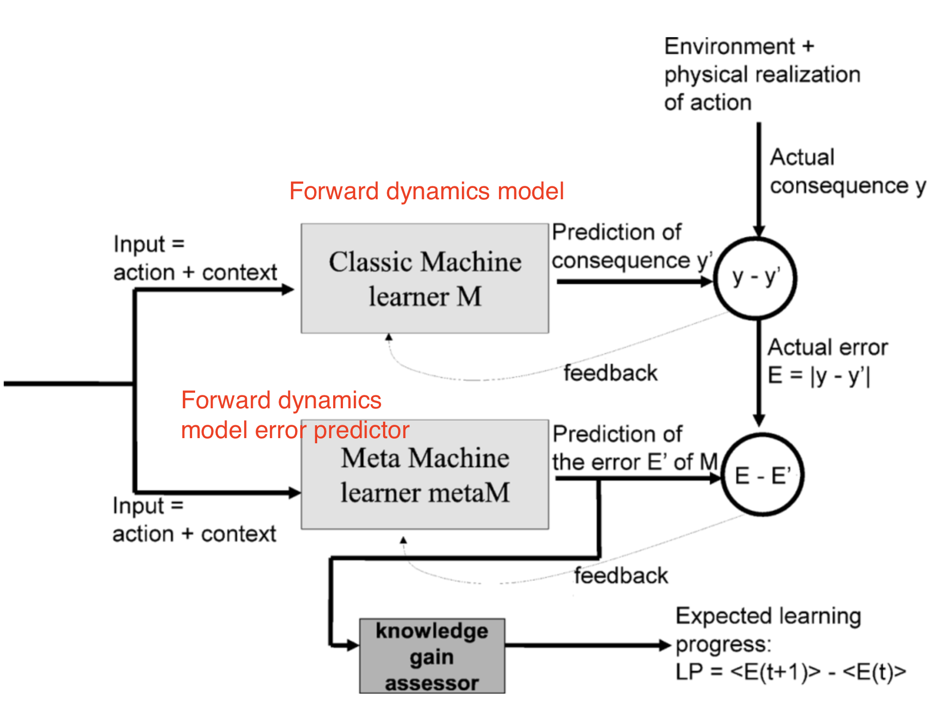
Intelligent Adaptive Curiosity (IAC; Oudeyer, et al. 2007) sketched an idea of using a forward dynamics prediction model to estimate learning progress and assigned intrinsic exploration reward accordingly.

IAC relies on a memory which stores all the experiences encountered by the robot, $M=\{(s_t, a_t, s_{t+1})\}$ and a forward dynamics model $f$. IAC incrementally splits the state space (i.e. sensorimotor space in the context of robotics, as discussed in the paper) into separate regions based on the transition samples, using a process similar to how a decision tree is split: The split happens when the number of samples is larger than a threshold, and the variance of states in each leaf should be minimal. Each tree node is characterized by its exclusive set of samples and has its own forward dynamics predictor $f$, named “expert”.

The prediction error $e_t$ of an expert is pushed into a list associated with each region. The learning progress is then measured as the difference between the mean error rate of a moving window with offset $\tau$ and the current moving window. The intrinsic reward is defined for tracking the learning progress: $r^i_t = \frac{1}{k}\sum_{i=0}^{k-1}(e_{t-i-\tau} - e_{t-i})$, where $k$ is the moving window size. So the larger prediction error rate decrease we can achieve, the higher intrinsic reward we would assign to the agent. In other words, the agent is encouraged to take actions to quickly learn about the environment.

Stadie et al. (2015) trained a forward dynamics model in the encoding space defined by $\phi$, $f_\phi: (\phi(s_t), a_t) \mapsto \phi(s_{t+1})$. The model’s prediction error at time $T$ is normalized by the maximum error up to time $t$, $\bar{e}_t = \frac{e_t}{\max_{i \leq t} e_i}$, so it is always between 0 and 1. The intrinsic reward is defined accordingly: $r^i_t = (\frac{\bar{e}_t(s_t, a_t)}{t \cdot C})$, where $C > 0$ is a decay constant.

Encoding the state space via $\phi(.)$ is necessary, as experiments in the paper have shown that a dynamics model trained directly on raw pixels has very poor behavior — assigning same exploration bonuses to all the states. In Stadie et al. (2015), the encoding function $\phi$ is learned via an autocoder (AE) and $\phi(.)$ is one of the output layers in AE. The AE can be statically trained using a set of images collected by a random agent, or dynamically trained together with the policy where the early frames are gathered using $\epsilon$-greedy exploration.

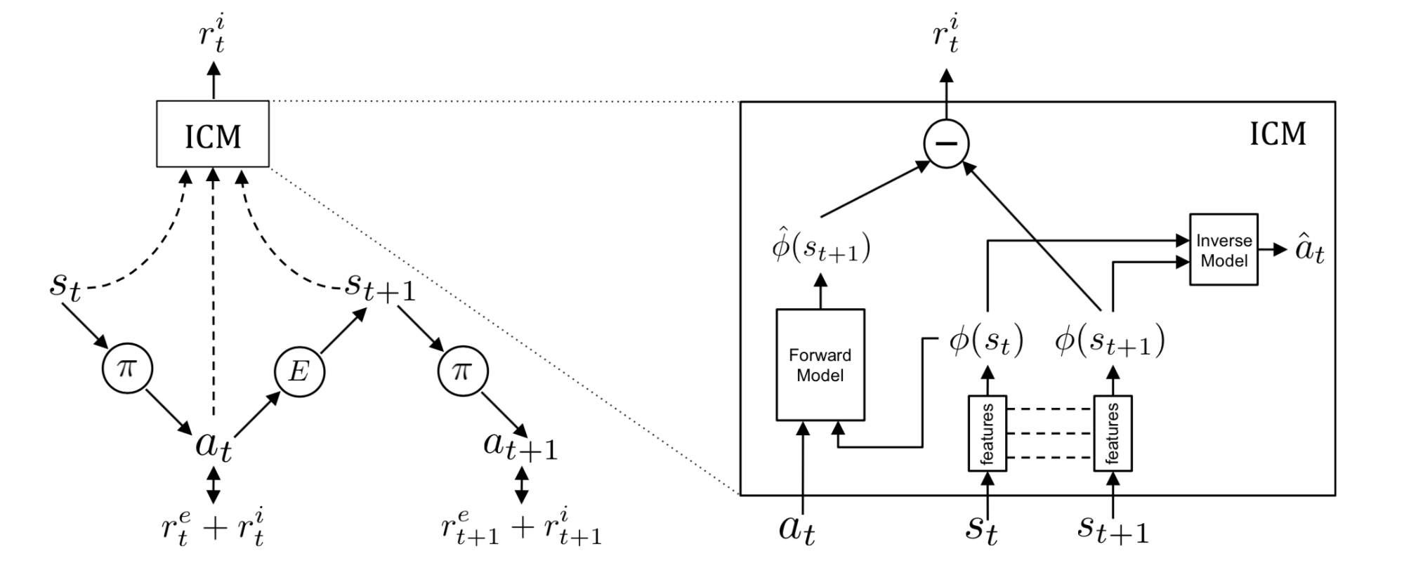
Instead of autoencoder, Intrinsic Curiosity Module (ICM; Pathak, et al., 2017) learns the state space encoding $\phi(.)$ with a self-supervised inverse dynamics model. Predicting the next state given the agent’s own action is not easy, especially considering that some factors in the environment cannot be controlled by the agent or do not affect the agent. ICM believes that a good state feature space should exclude such factors because they cannot influence the agent’s behavior and thus the agent has no incentive for learning them. By learning an inverse dynamics model $g: (\phi(s_t), \phi(s_{t+1})) \mapsto a_t$, the feature space only captures those changes in the environment related to the actions of our agent, and ignores the rest.

Given a forward model $f$, an inverse dynamics model $g$ and an observation $(s_t, a_t, s_{t+1})$:

Such $\phi(.)$ is expected to be robust to uncontrollable aspects of the environment.

Burda, Edwards & Pathak, et al. (2018) did a set of large-scale comparison experiments on purely curiosity-driven learning, meaning that only intrinsic rewards are provided to the agent. In this study, the reward is $r_t = r^i_t = | f(s_t, a_t) - \phi(s_{t+1})|_2^2$. A good choice of $\phi$ is crucial to learning forward dynamics, which is expected to be compact, sufficient and stable, making the prediction task more tractable and filtering out irrelevant observation.

In comparison of 4 encoding functions:

1. Raw image pixels: No encoding, $\phi(x) = x$.
2. Random features (RF): Each state is compressed through a fixed random neural network.
3. VAE: The probabilistic encoder is used for encoding, $\phi(x) = q(z \vert x)$.
4. Inverse dynamic features (IDF): The same feature space as used in ICM.

All the experiments have the reward signals normalized by a running estimation of standard deviation of the cumulative returns. And all the experiments are running in an infinite horizon setting to avoid “done” flag leaking information.

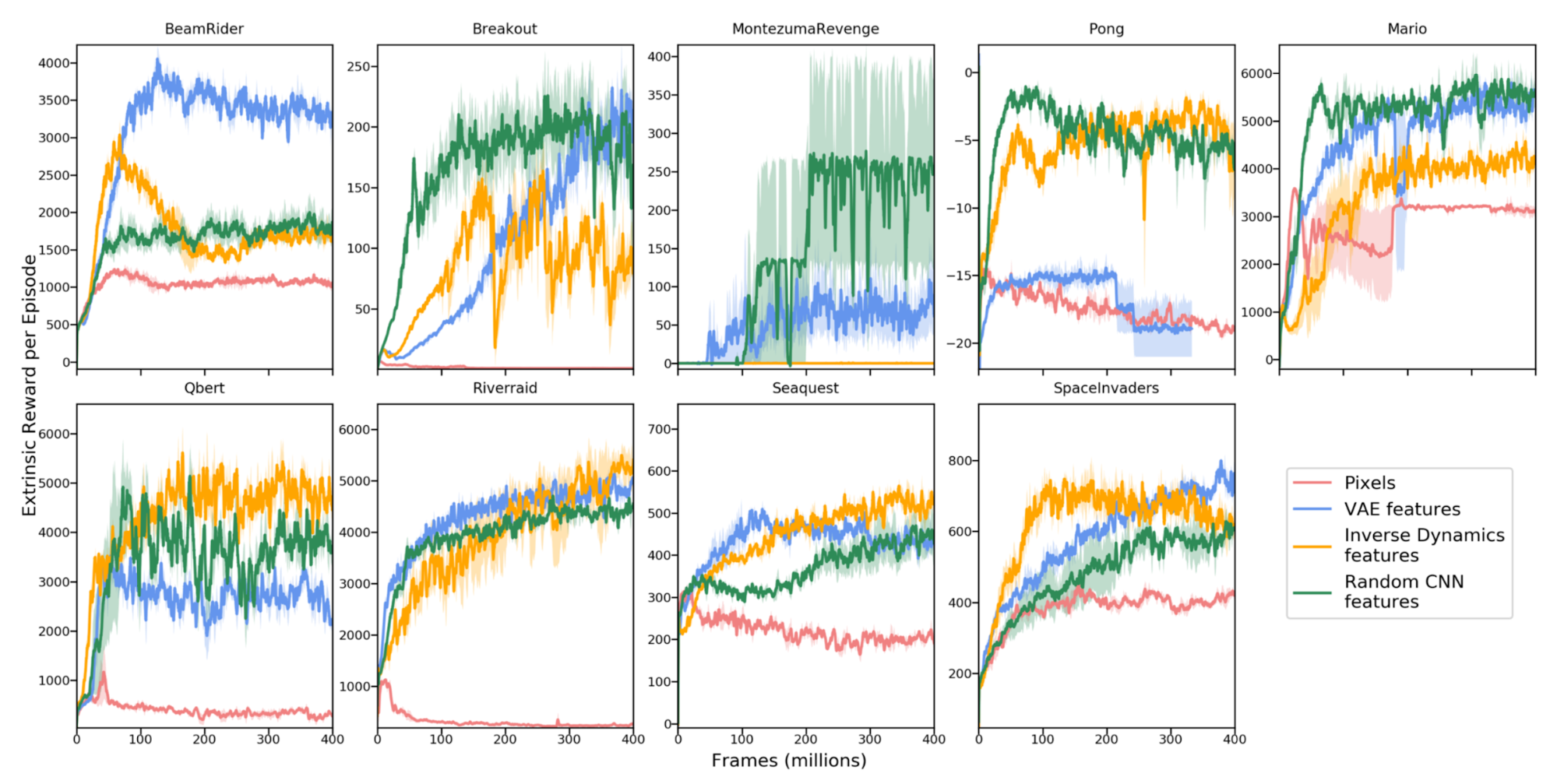
Interestingly random features turn out to be quite competitive, but in feature transfer experiments (i.e. train an agent in Super Mario Bros level 1-1 and then test it in another level), learned IDF features can generalize better.

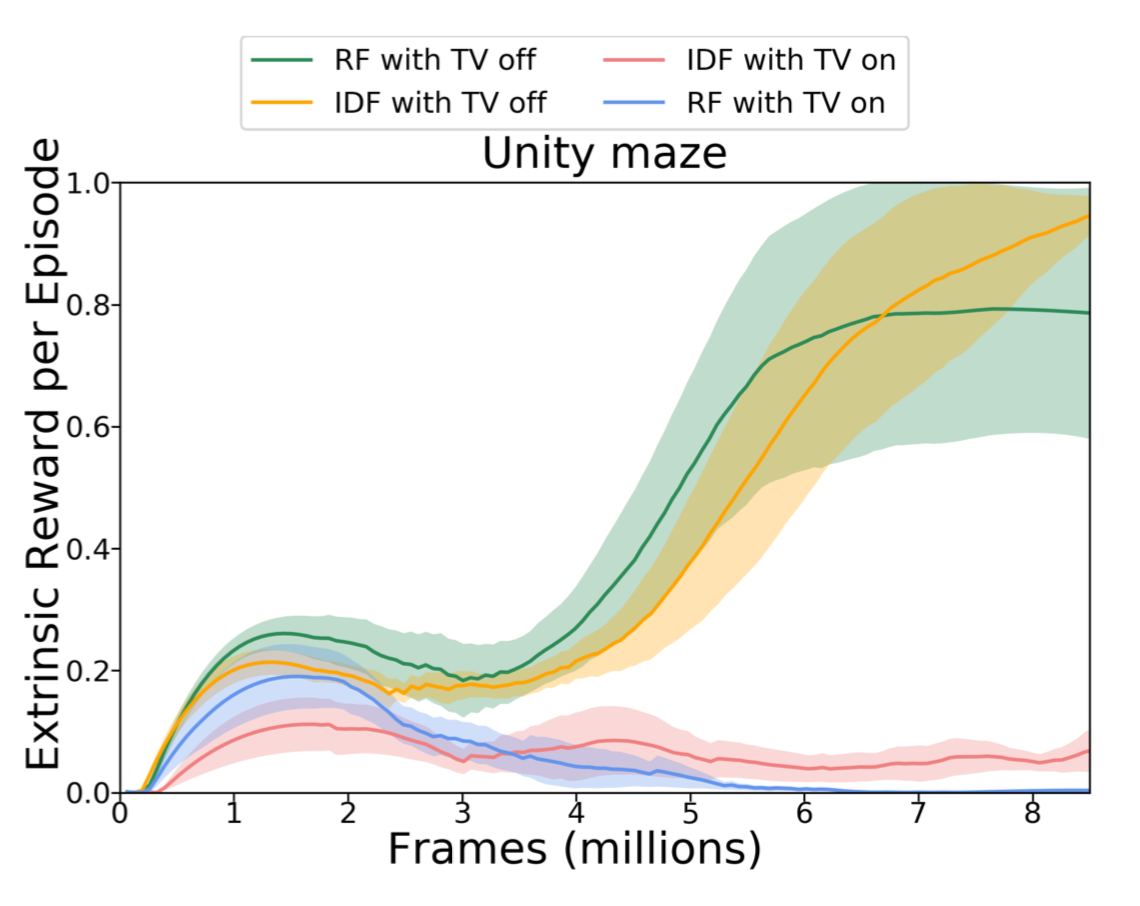
They also compared RF and IDF in an environment with a noisy TV on. Unsurprisingly the noisy TV drastically slows down the learning and extrinsic rewards are much lower in time.

The forward dynamics optimization can be modeled via variational inference as well. VIME (short for “Variational information maximizing exploration”; Houthooft, et al. 2017) is an exploration strategy based on maximization of information gain about the agent’s belief of environment dynamics. How much additional information has been obtained about the forward dynamics can be measured as the reduction in entropy.

Let $\mathcal{P}$ be the environment transition function, $p(s_{t+1}\vert s_t, a_t; \theta)$ be the forward prediction model, parameterized by $\theta \in \Theta$, and $\xi_t = \{s_1, a_1, \dots, s_t\}$ be the trajectory history. We would like to reduce the entropy after taking a new action and observing the next state, which is to maximize the following:

While taking expectation over the new possible states, the agent is expected to take a new action to increase the KL divergence (“information gain”) between its new belief over the prediction model to the old one. This term can be added into the reward function as an intrinsic reward: $r^i_t = D_\text{KL} [p(\theta \vert \xi_t, a_t, s_{t+1}) | p(\theta \vert \xi_t))]$.

However, computing the posterior $p(\theta \vert \xi_t, a_t, s_{t+1})$ is generally intractable.

Since it is difficult to compute $p(\theta\vert\xi_t)$ directly, a natural choice is to approximate it with an alternative distribution $q_\phi(\theta)$. With variational lower bound, we know the maximization of $q_\phi(\theta)$ is equivalent to maximizing $p(\xi_t\vert\theta)$ and minimizing $D_\text{KL}[q_\phi(\theta) | p(\theta)]$.

Using the approximation distribution $q$, the intrinsic reward becomes:

where $\phi_{t+1}$ represents $q$’s parameters associated with the new relief after seeing $a_t$ and $s_{t+1}$. When used as an exploration bonus, it is normalized by division by the moving median of this KL divergence value.

Here the dynamics model is parameterized as a Bayesian neural network (BNN), as it maintains a distribution over its weights. The BNN weight distribution $q_\phi(\theta)$ is modeled as a fully factorized Gaussian with $\phi = \{\mu, \sigma\}$ and we can easily sample $\theta \sim q_\phi(.)$. After applying a second-order Taylor expansion, the KL term $D_\text{KL}[q_{\phi + \lambda \Delta\phi}(\theta) | q_{\phi}(\theta)]$ can be estimated using Fisher Information Matrix $\mathbf{F}_\phi$, which is easy to compute, because $q_\phi$ is factorized Gaussian and thus the covariance matrix is only a diagonal matrix. See more details in the paper, especially section 2.3-2.5.

All the methods above depend on a single prediction model. If we have multiple such models, we could use the disagreement among models to set the exploration bonus (Pathak, et al. 2019). High disagreement indicates low confidence in prediction and thus requires more exploration. Pathak, et al. (2019) proposed to train a set of forward dynamics models and to use the variance over the ensemble of model outputs as $r_t^i$. Precisely, they encode the state space with random feature and learn 5 models in the ensemble.

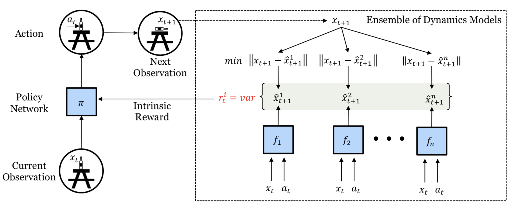
Because $r^i_t$ is differentiable, the intrinsic reward in the model could be directly optimized through gradient descent so as to inform the policy agent to change actions. This differentiable exploration approach is very efficient but limited by having a short exploration horizon.

Random Networks

But, what if the prediction task is not about the environment dynamics at all? It turns out when the prediction is for a random task, it still can help exploration.

DORA (short for “Directed Outreaching Reinforcement Action-Selection”; Fox & Choshen, et al. 2018) is a novel framework that injects exploration signals based on a newly introduced, task-independent MDP. The idea of DORA depends on two parallel MDPs:

• One is the original task MDP;
• The other is an identical MDP but with no reward attached: Rather, every state-action pair is designed to have value 0. The Q-value learned for the second MDP is called E-value. If the model cannot perfectly predict E-value to be zero, it is still missing information.

Initially E-value is assigned with value 1. Such positive initialization can encourage directed exploration for better E-value prediction. State-action pairs with high E-value estimation don’t have enough information gathered yet, at least not enough to exclude their high E-values. To some extent, the logarithm of E-values can be considered as a generalization of visit counters.

When using a neural network to do function approximation for E-value, another value head is added to predict E-value and it is simply expected to predict zero. Given a predicted E-value $E(s_t, a_t)$, the exploration bonus is $r^i_t = \frac{1}{\sqrt{-\log E(s_t, a_t)}}$.

Similar to DORA, Random Network Distillation (RND; Burda, et al. 2018) introduces a prediction task independent of the main task. The RND exploration bonus is defined as the error of a neural network $\hat{f}(s_t)$ predicting features of the observations given by a fixed randomly initialized neural network $f(s_t)$. The motivation is that given a new state, if similar states have been visited many times in the past, the prediction should be easier and thus has lower error. The exploration bonus is $r^i(s_t) = |\hat{f}(s_t; \theta) - f(s_t) |_2^2$.

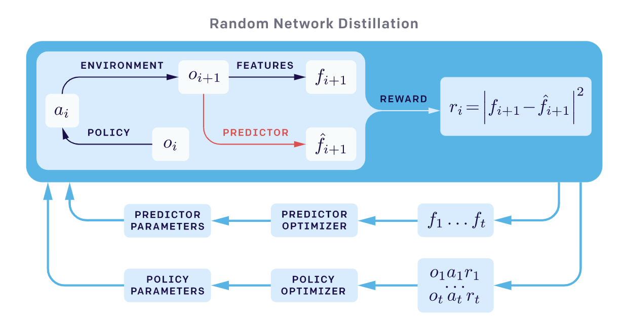
Two factors are important in RND experiments:

1. Non-episodic setting results in better exploration, especially when not using any extrinsic rewards. It means that the return is not truncated at “Game over” and intrinsic return can spread across multiple episodes.
2. Normalization is important since the scale of the reward is tricky to adjust given a random neural network as a prediction target. The intrinsic reward is normalized by division by a running estimate of the standard deviations of the intrinsic return.

The RND setup works well for resolving the hard-exploration problem. For example, maximizing the RND exploration bonus consistently finds more than half of the rooms in Montezuma’s Revenge.

Physical Properties

Different from games in simulators, some RL applications like Robotics need to understand objects and intuitive reasoning in the physical world. Some prediction tasks require the agent to perform a sequence of interactions with the environment and to observe the corresponding consequences, such as estimating some hidden properties in physics (e.g. mass, friction, etc).

Motivated by such ideas, Denil, et al. (2017) found that DRL agents can learn to perform necessary exploration to discover such hidden properties. Precisely they considered two experiments:

1. “Which is heavier?” — The agent has to interact with the blocks and infer which one is heavier.
2. “Towers” — The agent needs to infer how many rigid bodies a tower is composed of by knocking it down.

The agent in the experiments first goes through an exploration phase to interact with the environment and to collect information. Once the exploration phase ends, the agent is asked to output a labeling action to answer the question. Then a positive reward is assigned to the agent if the answer is correct; otherwise a negative one is assigned. Because the answer requires a decent amount of interactions with items in the scene, the agent has to learn to efficiently play around so as to figure out the physics and the correct answer. The exploration naturally happens.

In their experiments, the agent is able to learn in both tasks with performance varied by the difficulty of the task. Although the paper didn’t use the physics prediction task to provide intrinsic reward bonus along with extrinsic reward associated with another learning task, rather it focused on the exploration tasks themselves. I do enjoy the idea of encouraging sophisticated exploration behavior by predicting hidden physics properties in the environment.

Memory-based Exploration

Reward-based exploration suffers from several drawbacks:

• Function approximation is slow to catch up.
• Exploration bonus is non-stationary.
• Knowledge fading, meaning that states cease to be novel and cannot provide intrinsic reward signals in time.

Methods in this section rely on external memory to resolve disadvantages of reward bonus-based exploration.

Episodic Memory

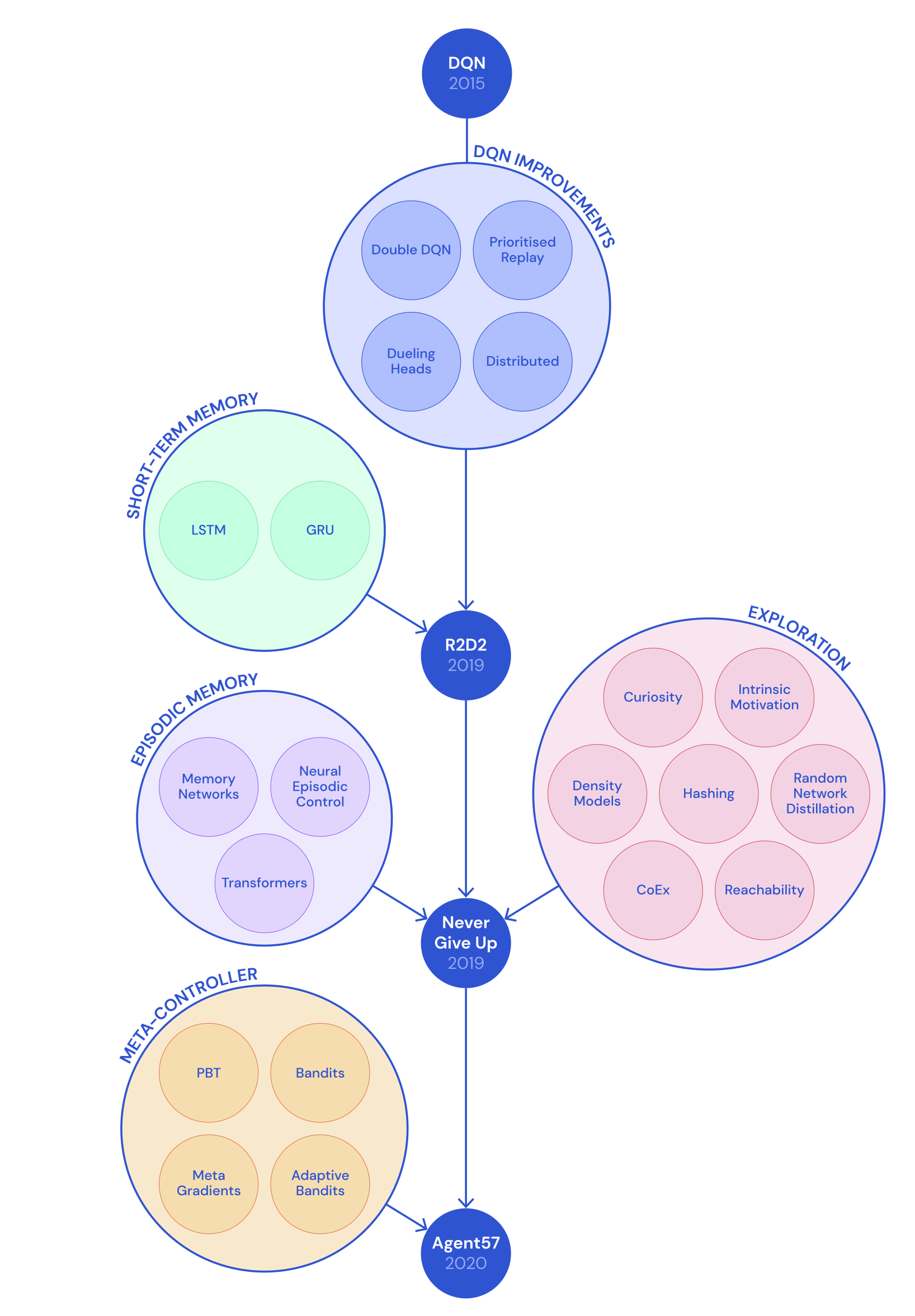
As mentioned above, RND is better running in an non-episodic setting, meaning the prediction knowledge is accumulated across multiple episodes. The exploration strategy, Never Give Up (NGU; Badia, et al. 2020a), combines an episodic novelty module that can rapidly adapt within one episode with RND as a lifelong novelty module.

Precisely, the intrinsic reward in NGU consists of two exploration bonuses from two modules, within one episode and across multiple episodes, respectively.

The short-term per-episode reward is provided by an episodic novelty module. It contains an episodic memory $M$, a dynamically-sized slot-based memory, and an IDF (inverse dynamics features) embedding function $\phi$, same as the feature encoding in ICM

1. At every step the current state embedding $\phi(s_t)$ is added into $M$.

2. The intrinsic bonus is determined by comparing how similar the current observation is to the content of $M$. A larger difference results in a larger bonus.

   $$ r^\text{episodic}_t \approx \frac{1}{\sqrt{\sum_{\phi_i \in N_k} K(\phi(x_t), \phi_i)} + c} $$

   where $K(x, y)$ is a kernel function for measuring the distance between two samples. $N_k$ is a set of $k$ nearest neighbors in $M$ according to $K(., .)$. $c$ is a small constant to keep the denominator non-zero. In the paper, $K(x, y)$ is configured to be the inverse kernel:

   $$ K(x, y) = \frac{\epsilon}{\frac{d^2(x, y)}{d^2_m} + \epsilon} $$

   where $d(.,.)$ is Euclidean distance between two samples and $d_m$ is a running average of the squared Euclidean distance of the k-th nearest neighbors for better robustness. $\epsilon$ is a small constant.

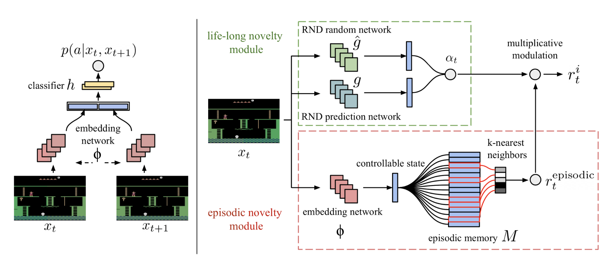
The long-term across-episode novelty relies on RND prediction error in life-long novelty module. The exploration bonus is $\alpha_t = 1 + \frac{e^\text{RND}(s_t) - \mu_e}{\sigma_e}$ where $\mu_e$ and $\sigma_e$ are running mean and std dev for RND error $e^\text{RND}(s_t)$.

However in the conclusion section of the RND paper, I noticed the following statement:

“We find that the RND exploration bonus is sufficient to deal with local exploration, i.e. exploring the consequences of short-term decisions, like whether to interact with a particular object, or avoid it. However global exploration that involves coordinated decisions over long time horizons is beyond the reach of our method. "

And this confuses me a bit how RND can be used as a good life-long novelty bonus provider. If you know why, feel free to leave a comment below.

The final combined intrinsic reward is $r^i_t = r^\text{episodic}_t \cdot \text{clip}(\alpha_t, 1, L)$, where $L$ is a constant maximum reward scalar.

The design of NGU enables it to have two nice properties:

1. Rapidly discourages revisiting the same state within the same episode;
2. Slowly discourages revisiting states that have been visited many times across episodes.

Later, built on top of NGU, DeepMind proposed “Agent57” (Badia, et al. 2020b), the first deep RL agent that outperforms the standard human benchmark on all 57 Atari games. Two major improvements in Agent57 over NGU are:

1. A population of policies are trained in Agent57, each equipped with a different exploration parameter pair $\{(\beta_j, \gamma_j)\}_{j=1}^N$. Recall that given $\beta_j$, the reward is constructed as $r_{j,t} = r_t^e + \beta_j r^i_t$ and $\gamma_j$ is the reward discounting factor. It is natural to expect policies with higher $\beta_j$ and lower $\gamma_j$ to make more progress early in training, while the opposite would be expected as training progresses. A meta-controller (sliding-window UCB bandit algorithm) is trained to select which policies should be prioritized.
2. The second improvement is a new parameterization of Q-value function that decomposes the contributions of the intrinsic and extrinsic rewards in a similar form as the bundled reward: $Q(s, a; \theta_j) = Q(s, a; \theta_j^e) + \beta_j Q(s, a; \theta_j^i)$. During training, $Q(s, a; \theta_j^e)$ and $Q(s, a; \theta_j^i)$ are optimized separately with rewards $r_j^e$ and $r_j^i$, respectively.

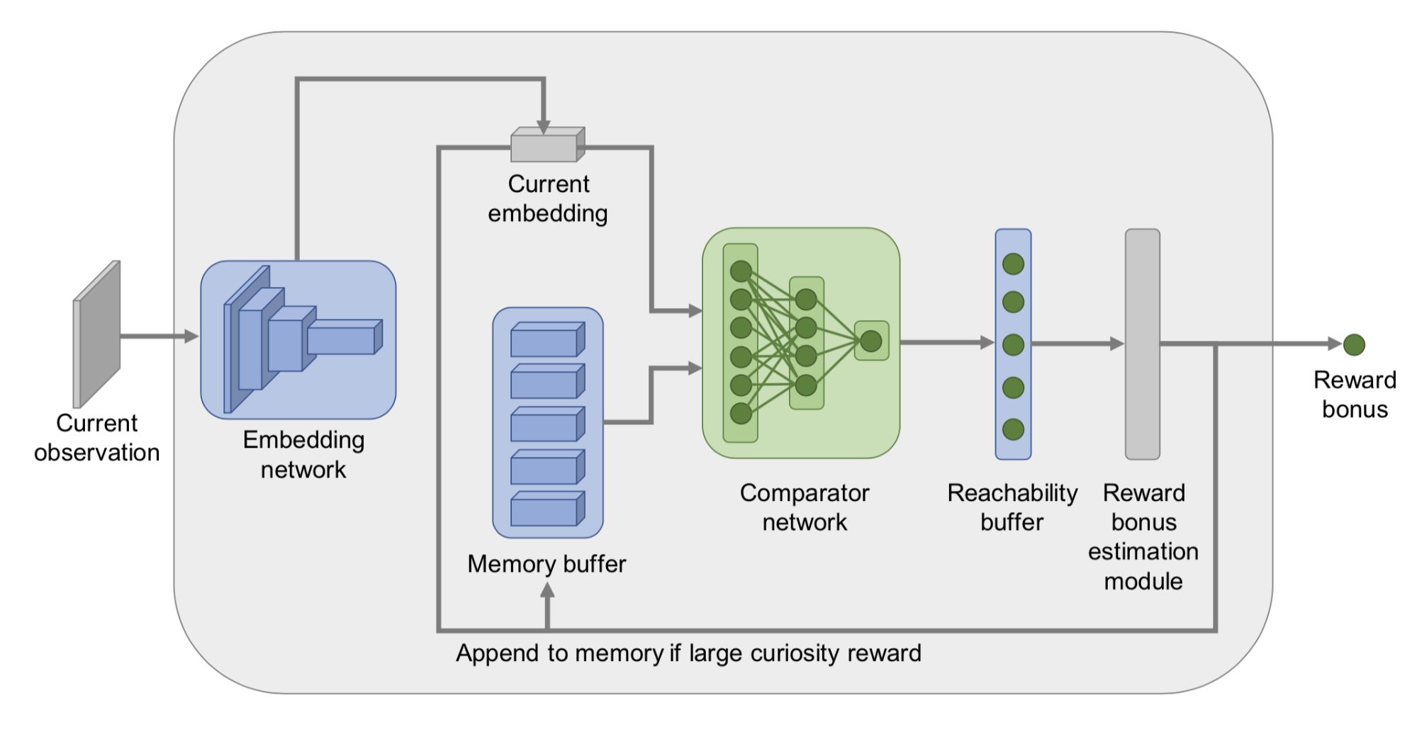
Instead of using the Euclidean distance to measure closeness of states in episodic memory, Savinov, et al. (2019) took the transition between states into consideration and proposed a method to measure the number of steps needed to visit one state from other states in memory, named Episodic Curiosity (EC) module. The novelty bonus depends on reachability between states.

1. At the beginning of each episode, the agent starts with an empty episodic memory $M$.
2. At every step, the agent compares the current state with saved states in memory to determine novelty bonus: If the current state is novel (i.e., takes more steps to reach from observations in memory than a threshold), the agent gets a bonus.
3. The current state is added into the episodic memory if the novelty bonus is high enough. (Imagine that if all the states were added into memory, any new state could be added within 1 step.)
4. Repeat 1-3 until the end of this episode.

In order to estimate reachability between states, we need to access the transition graph, which is unfortunately not entirely known. Thus, Savinov, et al. (2019) trained a siamese neural network to predict how many steps separate two states. It contains one embedding network $\phi: \mathcal{S} \mapsto \mathbb{R}^n$ to first encode the states to feature vectors and then one comparator network $C: \mathbb{R}^n \times \mathbb{R}^n \mapsto [0, 1]$ to output a binary label on whether two states are close enough (i.e., reachable within $k$ steps) in the transition graph, $C(\phi(s_i), \phi(s_j)) \mapsto [0, 1]$.

An episodic memory buffer $M$ stores embeddings of some past observations within the same episode. A new observation will be compared with existing state embeddings via $C$ and the results are aggregated (e.g. max, 90th percentile) to provide a reachability score $C^M(\phi(s_t))$. The exploration bonus is $r^i_t = \big(C’ - C^M(f(s_t))\big)$, where $C’$ is a predefined threshold for determining the sign of the reward (e.g. $C’=0.5$ works well for fixed-duration episodes). High bonus is awarded to new states when they are not easily reachable from states in the memory buffer.

They claimed that the EC module can overcome the noisy-TV problem.

Direct Exploration

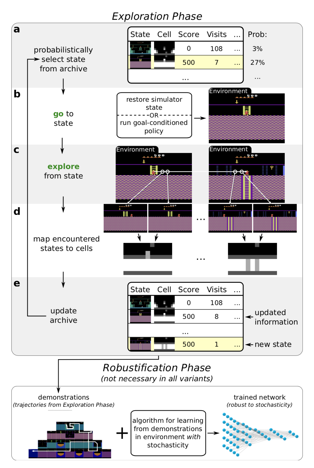
Go-Explore (Ecoffet, et al., 2019) is an algorithm aiming to solve the “hard-exploration” problem. It is composed of the following two phases.

Phase 1 (“Explore until solved”) feels quite like Dijkstra’s algorithm for finding shortest paths in a graph. Indeed, no neural network is involved in phase 1. By maintaining a memory of interesting states as well as trajectories leading to them, the agent can go back (given a simulator is deterministic) to promising states and continue doing random exploration from there. The state is mapped into a short discretized code (named “cell”) in order to be memorized. The memory is updated if a new state appears or a better/shorter trajectory is found. When selecting which past states to return to, the agent might select one in the memory uniformly or according to heuristics like recency, visit count, count of neighbors in the memory, etc. This process is repeated until the task is solved and at least one solution trajectory is found.

The above found high-performance trajectories would not work well on evaluation envs with any stochasticity. Thus, Phase 2 (“Robustification”) is needed to robustify the solution via imitation learning. They adopted Backward Algorithm, in which the agent is started near the last state in the trajectory and then runs RL optimization from there.

One important note in phase 1 is: In order to go back to a state deterministically without exploration, Go-Explore depends on a resettable and deterministic simulator, which is a big disadvantage.

To make the algorithm more generally useful to environments with stochasticity, an enhanced version of Go-Explore (Ecoffet, et al., 2020), named policy-based Go-Explore was proposed later.

• Instead of resetting the simulator state effortlessly, the policy-based Go-Explore learns a goal-conditioned policy and uses that to access a known state in memory repeatedly. The goal-conditioned policy is trained to follow the best trajectory that previously led to the selected states in memory. They include a Self-Imitation Learning (SIL; Oh, et al. 2018) loss to help extract as much information as possible from successful trajectories.
• Also, they found sampling from policy works better than random actions when the agent returns to promising states to continue exploration.
• Another improvement in policy-based Go-Explore is to make the downscaling function of images to cells adjustable. It is optimized so that there would be neither too many nor too few cells in the memory.

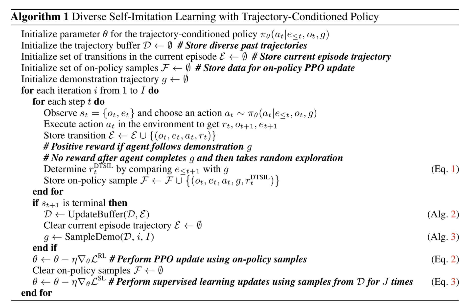
After vanilla Go-Explore, Yijie Guo, et al. (2019) proposed DTSIL (Diverse Trajectory-conditioned Self-Imitation Learning), which shared a similar idea as policy-based Go-Explore above. DTSIL maintains a memory of diverse demonstrations collected during training and uses them to train a trajectory-conditioned policy via SIL. They prioritize trajectories that end with a rare state during sampling.

The similar approach is also seen in Guo, et al. (2019). The main idea is to store goals with high uncertainty in memory so that later the agent can revisit these goal states with a goal-conditioned policy repeatedly. In each episode, the agent flips a coin (probability 0.5) to decide whether it will act greedily w.r.t. the policy or do directed exploration by sampling goals from the memory.

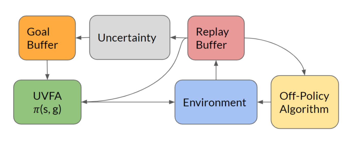
The uncertainty measure of a state can be something simple like count-based bonuses or something complex like density or bayesian models. The paper trained a forward dynamics model and took its prediction error as the uncertainty metric.

Q-Value Exploration

Inspired by Thompson sampling, Bootstrapped DQN (Osband, et al. 2016) introduces a notion of uncertainty in Q-value approximation in classic DQN by using the bootstrapping method. Bootstrapping is to approximate a distribution by sampling with replacement from the same population multiple times and then aggregate the results.

Multiple Q-value heads are trained in parallel but each only consumes a bootstrapped sub-sampled set of data and each has its own corresponding target network. All the Q-value heads share the same backbone network.

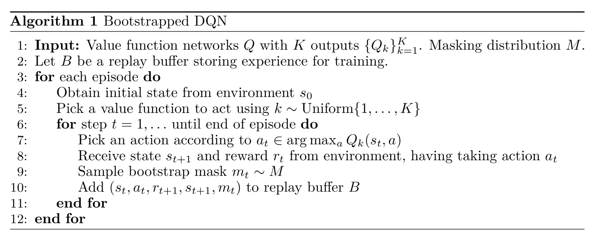
At the beginning of one episode, one Q-value head is sampled uniformly and acts for collecting experience data in this episode. Then a binary mask is sampled from the masking distribution $m \sim \mathcal{M}$ and decides which heads can use this data for training. The choice of masking distribution $\mathcal{M}$ determines how bootstrapped samples are generated; For example,

• If $\mathcal{M}$ is an independent Bernoulli distribution with $p=0.5$, this corresponds to the double-or-nothing bootstrap.
• If $\mathcal{M}$ always returns an all-one mask, the algorithm reduces to an ensemble method.

However, this kind of exploration is still restricted, because uncertainty introduced by bootstrapping fully relies on the training data. It is better to inject some prior information independent of the data. This “noisy” prior is expected to drive the agent to keep exploring when the reward is sparse. The algorithm of adding random prior into bootstrapped DQN for better exploration (Osband, et al. 2018) depends on Bayesian linear regression. The core idea of Bayesian regression is: We can “generate posterior samples by training on noisy versions of the data, together with some random regularization”.

Let $\theta$ be the Q function parameter and $\theta^-$ for the target Q, the loss function using a randomized prior function $p$ is:

Varitional Options

Options are policies with termination conditions. There are a large set of options available in the search space and they are independent of an agent’s intentions. By explicitly including intrinsic options into modeling, the agent can obtain intrinsic rewards for exploration.

VIC (short for “Variational Intrinsic Control”; Gregor, et al. 2017) is such a framework for providing the agent with intrinsic exploration bonuses based on modeling options and learning policies conditioned on options. Let $\Omega$ represent an option which starts from $s_0$ and ends at $s_f$. An environment probability distribution $p^J(s_f \vert s_0, \Omega)$ defines where an option $\Omega$ terminates given a starting state $s_0$. A controllability distribution $p^C(\Omega \vert s_0)$ defines the probability distribution of options we can sample from. And by definition we have $p(s_f, \Omega \vert s_0) = p^J(s_f \vert s_0, \Omega) p^C(\Omega \vert s_0)$.

While choosing options, we would like to achieve two goals:

• Achieve a diverse set of the final states from $s_0$ ⇨ Maximization of $H(s_f \vert s_0)$.
• Know precisely which state a given option $\Omega$ can end with ⇨ Minimization of $H(s_f \vert s_0, \Omega)$.

Combining them, we get mutual information $I(\Omega; s_f \vert s_0)$ to maximize:

Because mutual information is symmetric, we can switch $s_f$ and $\Omega$ in several places without breaking the equivalence. Also because $p(\Omega \vert s_0, s_f)$ is difficult to observe, let us replace it with an approximation distribution $q$. According to the variational lower bound, we would have $I(\Omega; s_f \vert s_0) \geq I^{VB}(\Omega; s_f \vert s_0)$.

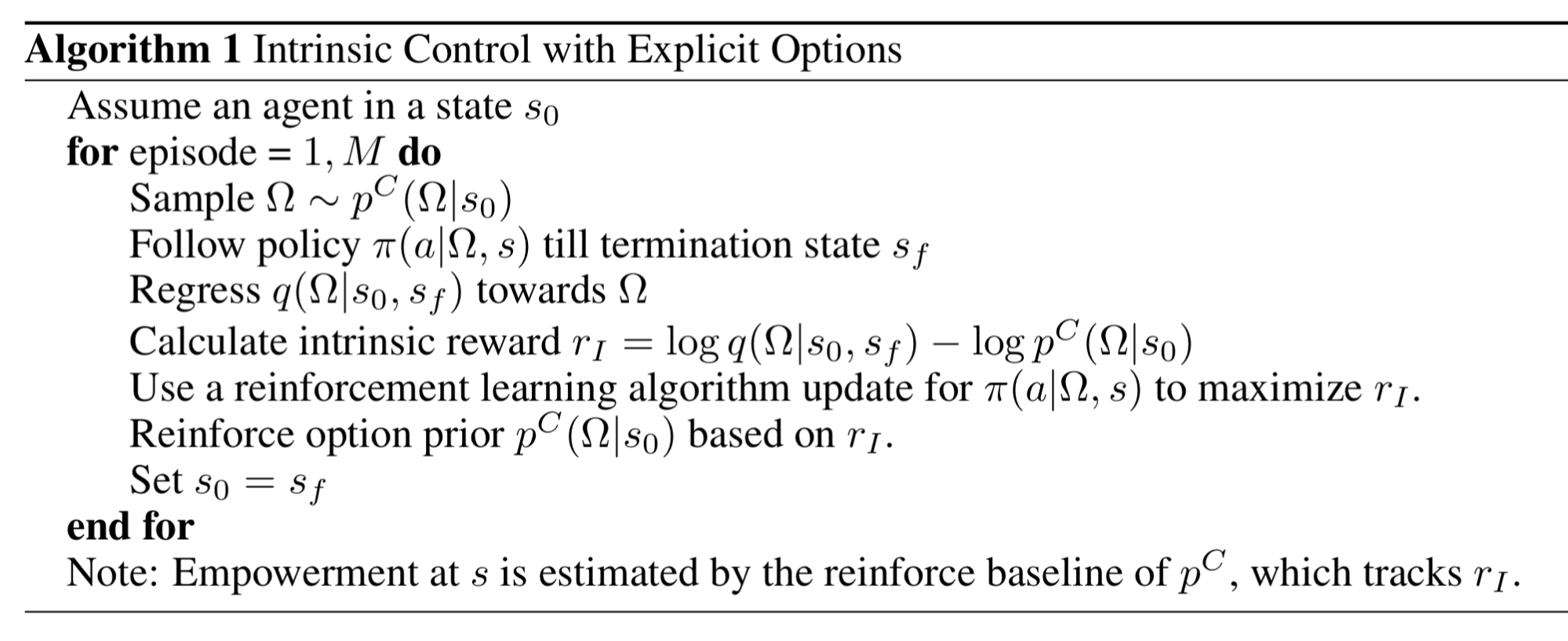
Here $\pi(a \vert \Omega, s)$ can be optimized with any RL algorithm. The option inference function $q(\Omega \vert s_0, s_f)$ is doing supervised learning. The prior $p^C$ is updated so that it tends to choose $\Omega$ with higher rewards. Note that $p^C$ can also be fixed (e.g. a Gaussian). Various $\Omega$ will result in different behavior through learning. Additionally, Gregor, et al. (2017) observed that it is difficult to make VIC with explicit options work in practice with function approximation and therefore they also proposed another version of VIC with implicit options.

Different from VIC which models $\Omega$ conditioned only on the start and end states, VALOR (short for “Variational Auto-encoding Learning of Options by Reinforcement”; Achiam, et al. 2018) relies on the whole trajectory to extract the option context $c$, which is sampled from a fixed Gaussian distribution. In VALOR:

• A policy acts as an encoder, translating contexts from a noise distribution into trajectories
• A decoder attempts to recover the contexts from the trajectories, and rewards the policies for making contexts easier to distinguish. The decoder never sees the actions during training, so the agent has to interact with the environment in a way that facilitates communication with the decoder for better prediction. Also, the decoder recurrently takes in a sequence of steps in one trajectory to better model the correlation between timesteps.

DIAYN (“Diversity is all you need”; Eysenbach, et al. 2018) has the idea lying in the same direction, although with a different name — DIAYN models the policies conditioned on a latent skill variable. See my previous post for more details.

Citation

Cited as:

Weng, Lilian. (Jun 2020). Exploration strategies in deep reinforcement learning. Lil’Log. https://lilianweng.github.io/posts/2020-06-07-exploration-drl/.

Or

@article{weng2020exploration,
  title   = "Exploration Strategies in Deep Reinforcement Learning",
  author  = "Weng, Lilian",
  journal = "lilianweng.github.io",
  year    = "2020",
  month   = "Jun",
  url     = "https://lilianweng.github.io/posts/2020-06-07-exploration-drl/"
}

Reference

[1] Pierre-Yves Oudeyer & Frederic Kaplan. “How can we define intrinsic motivation?” Conf. on Epigenetic Robotics, 2008.

[2] Marc G. Bellemare, et al. “Unifying Count-Based Exploration and Intrinsic Motivation”. NIPS 2016.

[3] Georg Ostrovski, et al. “Count-Based Exploration with Neural Density Models”. PMLR 2017.

[4] Rui Zhao & Volker Tresp. “Curiosity-Driven Experience Prioritization via Density Estimation”. NIPS 2018.

[5] Haoran Tang, et al. "#Exploration: A Study of Count-Based Exploration for Deep Reinforcement Learning”. NIPS 2017.

[6] Jürgen Schmidhuber. “A possibility for implementing curiosity and boredom in model-building neural controllers” 1991.

[7] Pierre-Yves Oudeyer, et al. “Intrinsic Motivation Systems for Autonomous Mental Development” IEEE Transactions on Evolutionary Computation, 2007.

[8] Bradly C. Stadie, et al. “Incentivizing Exploration In Reinforcement Learning With Deep Predictive Models”. ICLR 2016.

[9] Deepak Pathak, et al. “Curiosity-driven Exploration by Self-supervised Prediction”. CVPR 2017.

[10] Yuri Burda, Harri Edwards & Deepak Pathak, et al. “Large-Scale Study of Curiosity-Driven Learning”. arXiv 1808.04355 (2018).

[11] Joshua Achiam & Shankar Sastry. “Surprise-Based Intrinsic Motivation for Deep Reinforcement Learning” NIPS 2016 Deep RL Workshop.

[12] Rein Houthooft, et al. “VIME: Variational information maximizing exploration”. NIPS 2016.

[13] Leshem Choshen, Lior Fox & Yonatan Loewenstein. “DORA the explorer: Directed outreaching reinforcement action-selection”. ICLR 2018

[14] Yuri Burda, et al. “Exploration by Random Network Distillation” ICLR 2019.

[15] OpenAI Blog: “Reinforcement Learning with Prediction-Based Rewards” Oct, 2018.

[16] Misha Denil, et al. “Learning to Perform Physics Experiments via Deep Reinforcement Learning”. ICLR 2017.

[17] Ian Osband, et al. “Deep Exploration via Bootstrapped DQN”. NIPS 2016.

[18] Ian Osband, John Aslanides & Albin Cassirer. “Randomized Prior Functions for Deep Reinforcement Learning”. NIPS 2018.

[19] Karol Gregor, Danilo Jimenez Rezende & Daan Wierstra. “Variational Intrinsic Control”. ICLR 2017.

[20] Joshua Achiam, et al. “Variational Option Discovery Algorithms”. arXiv 1807.10299 (2018).

[21] Benjamin Eysenbach, et al. “Diversity is all you need: Learning skills without a reward function.”. ICLR 2019.

[22] Adrià Puigdomènech Badia, et al. “Never Give Up (NGU): Learning Directed Exploration Strategies” ICLR 2020.

[23] Adrià Puigdomènech Badia, et al. “Agent57: Outperforming the Atari Human Benchmark”. arXiv 2003.13350 (2020).

[24] DeepMind Blog: “Agent57: Outperforming the human Atari benchmark” Mar 2020.

[25] Nikolay Savinov, et al. “Episodic Curiosity through Reachability” ICLR 2019.

[26] Adrien Ecoffet, et al. “Go-Explore: a New Approach for Hard-Exploration Problems”. arXiv 1901.10995 (2019).

[27] Adrien Ecoffet, et al. “First return then explore”. arXiv 2004.12919 (2020).

[28] Junhyuk Oh, et al. “Self-Imitation Learning”. ICML 2018.

[29] Yijie Guo, et al. “Self-Imitation Learning via Trajectory-Conditioned Policy for Hard-Exploration Tasks”. arXiv 1907.10247 (2019).

[30] Zhaohan Daniel Guo & Emma Brunskill. “Directed Exploration for Reinforcement Learning”. arXiv 1906.07805 (2019).

[31] Deepak Pathak, et al. “Self-Supervised Exploration via Disagreement.” ICML 2019.