Stochastic gradient descent is a universal choice for optimizing deep learning models. However, it is not the only option. With black-box optimization algorithms, you can evaluate a target function $f(x): \mathbb{R}^n \to \mathbb{R}$, even when you don’t know the precise analytic form of $f(x)$ and thus cannot compute gradients or the Hessian matrix. Examples of black-box optimization methods include Simulated Annealing, Hill Climbing and Nelder-Mead method.
Evolution Strategies (ES) is one type of black-box optimization algorithms, born in the family of Evolutionary Algorithms (EA). In this post, I would dive into a couple of classic ES methods and introduce a few applications of how ES can play a role in deep reinforcement learning.
What are Evolution Strategies?
Evolution strategies (ES) belong to the big family of evolutionary algorithms. The optimization targets of ES are vectors of real numbers, $x \in \mathbb{R}^n$.
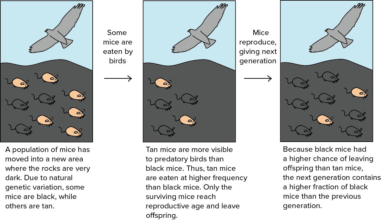
Evolutionary algorithms refer to a division of population-based optimization algorithms inspired by natural selection. Natural selection believes that individuals with traits beneficial to their survival can live through generations and pass down the good characteristics to the next generation. Evolution happens by the selection process gradually and the population grows better adapted to the environment.
Evolutionary algorithms can be summarized in the following format as a general optimization solution:
Let’s say we want to optimize a function $f(x)$ and we are not able to compute gradients directly. But we still can evaluate $f(x)$ given any $x$ and the result is deterministic. Our belief in the probability distribution over $x$ as a good solution to $f(x)$ optimization is $p_\theta(x)$, parameterized by $\theta$. The goal is to find an optimal configuration of $\theta$.
Here given a fixed format of distribution (i.e. Gaussian), the parameter $\theta$ carries the knowledge about the best solutions and is being iteratively updated across generations.
Starting with an initial value of $\theta$, we can continuously update $\theta$ by looping three steps as follows:
- Generate a population of samples $D = \{(x_i, f(x_i)\}$ where $x_i \sim p_\theta(x)$.
- Evaluate the “fitness” of samples in $D$.
- Select the best subset of individuals and use them to update $\theta$, generally based on fitness or rank.
In Genetic Algorithms (GA), another popular subcategory of EA, $x$ is a sequence of binary codes, $x \in \{0, 1\}^n$. While in ES, $x$ is just a vector of real numbers, $x \in \mathbb{R}^n$.
Simple Gaussian Evolution Strategies
This is the most basic and canonical version of evolution strategies. It models $p_\theta(x)$ as a $n$-dimensional isotropic Gaussian distribution, in which $\theta$ only tracks the mean $\mu$ and standard deviation $\sigma$.
The process of Simple-Gaussian-ES, given $x \in \mathcal{R}^n$:
- Initialize $\theta = \theta^{(0)}$ and the generation counter $t=0$
- Generate the offspring population of size $\Lambda$ by sampling from the Gaussian distribution:
$D^{(t+1)}=\{ x^{(t+1)}_i \mid x^{(t+1)}_i = \mu^{(t)} + \sigma^{(t)} y^{(t+1)}_i \text{ where } y^{(t+1)}_i \sim \mathcal{N}(x \vert 0, \mathbf{I}),;i = 1, \dots, \Lambda\}$
. - Select a top subset of $\lambda$ samples with optimal $f(x_i)$ and this subset is called elite set. Without loss of generality, we may consider the first $k$ samples in $D^{(t+1)}$ to belong to the elite group — Let’s label them as
- Then we estimate the new mean and std for the next generation using the elite set:
- Repeat steps (2)-(4) until the result is good enough ✌️
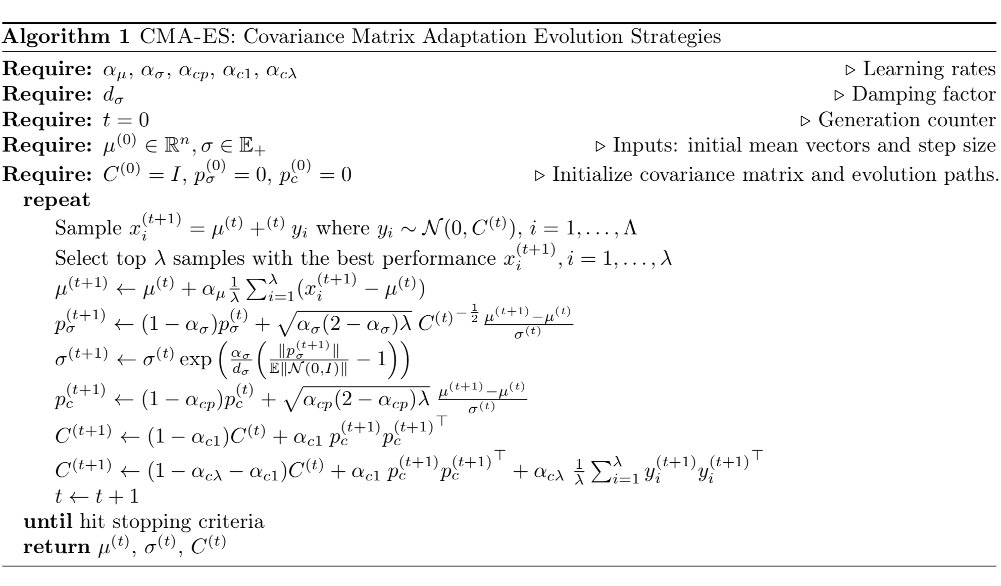
Covariance Matrix Adaptation Evolution Strategies (CMA-ES)
The standard deviation $\sigma$ accounts for the level of exploration: the larger $\sigma$ the bigger search space we can sample our offspring population. In vanilla ES, $\sigma^{(t+1)}$ is highly correlated with $\sigma^{(t)}$, so the algorithm is not able to rapidly adjust the exploration space when needed (i.e. when the confidence level changes).
CMA-ES, short for “Covariance Matrix Adaptation Evolution Strategy”, fixes the problem by tracking pairwise dependencies between the samples in the distribution with a covariance matrix $C$. The new distribution parameter becomes:
where $\sigma$ controls for the overall scale of the distribution, often known as step size.
Before we dig into how the parameters are updated in CMA-ES, it is better to review how the covariance matrix works in the multivariate Gaussian distribution first. As a real symmetric matrix, the covariance matrix $C$ has the following nice features (See proof & proof):
- It is always diagonalizable.
- Always positive semi-definite.
- All of its eigenvalues are real non-negative numbers.
- All of its eigenvectors are orthogonal.
- There is an orthonormal basis of $\mathbb{R}^n$ consisting of its eigenvectors.
Let the matrix $C$ have an orthonormal basis of eigenvectors $B = [b_1, \dots, b_n]$, with corresponding eigenvalues $\lambda_1^2, \dots, \lambda_n^2$. Let $D=\text{diag}(\lambda_1, \dots, \lambda_n)$.
The square root of $C$ is:
| Symbol | Meaning |
|---|---|
| $x_i^{(t)} \in \mathbb{R}^n$ | the $i$-th samples at the generation (t) |
| $y_i^{(t)} \in \mathbb{R}^n$ | $x_i^{(t)} = \mu^{(t-1)} + \sigma^{(t-1)} y_i^{(t)} $ |
| $\mu^{(t)}$ | mean of the generation (t) |
| $\sigma^{(t)}$ | step size |
| $C^{(t)}$ | covariance matrix |
| $B^{(t)}$ | a matrix of $C$’s eigenvectors as row vectors |
| $D^{(t)}$ | a diagonal matrix with $C$’s eigenvalues on the diagnose. |
| $p_\sigma^{(t)}$ | evaluation path for $\sigma$ at the generation (t) |
| $p_c^{(t)}$ | evaluation path for $C$ at the generation (t) |
| $\alpha_\mu$ | learning rate for $\mu$’s update |
| $\alpha_\sigma$ | learning rate for $p_\sigma$ |
| $d_\sigma$ | damping factor for $\sigma$’s update |
| $\alpha_{cp}$ | learning rate for $p_c$ |
| $\alpha_{c\lambda}$ | learning rate for $C$’s rank-min(λ, n) update |
| $\alpha_{c1}$ | learning rate for $C$’s rank-1 update |
Updating the Mean
CMA-ES has a learning rate $\alpha_\mu \leq 1$ to control how fast the mean $\mu$ should be updated. Usually it is set to 1 and thus the equation becomes the same as in vanilla ES, $\mu^{(t+1)} = \frac{1}{\lambda}\sum_{i=1}^\lambda (x_i^{(t+1)}$.
Controlling the Step Size
The sampling process can be decoupled from the mean and standard deviation:
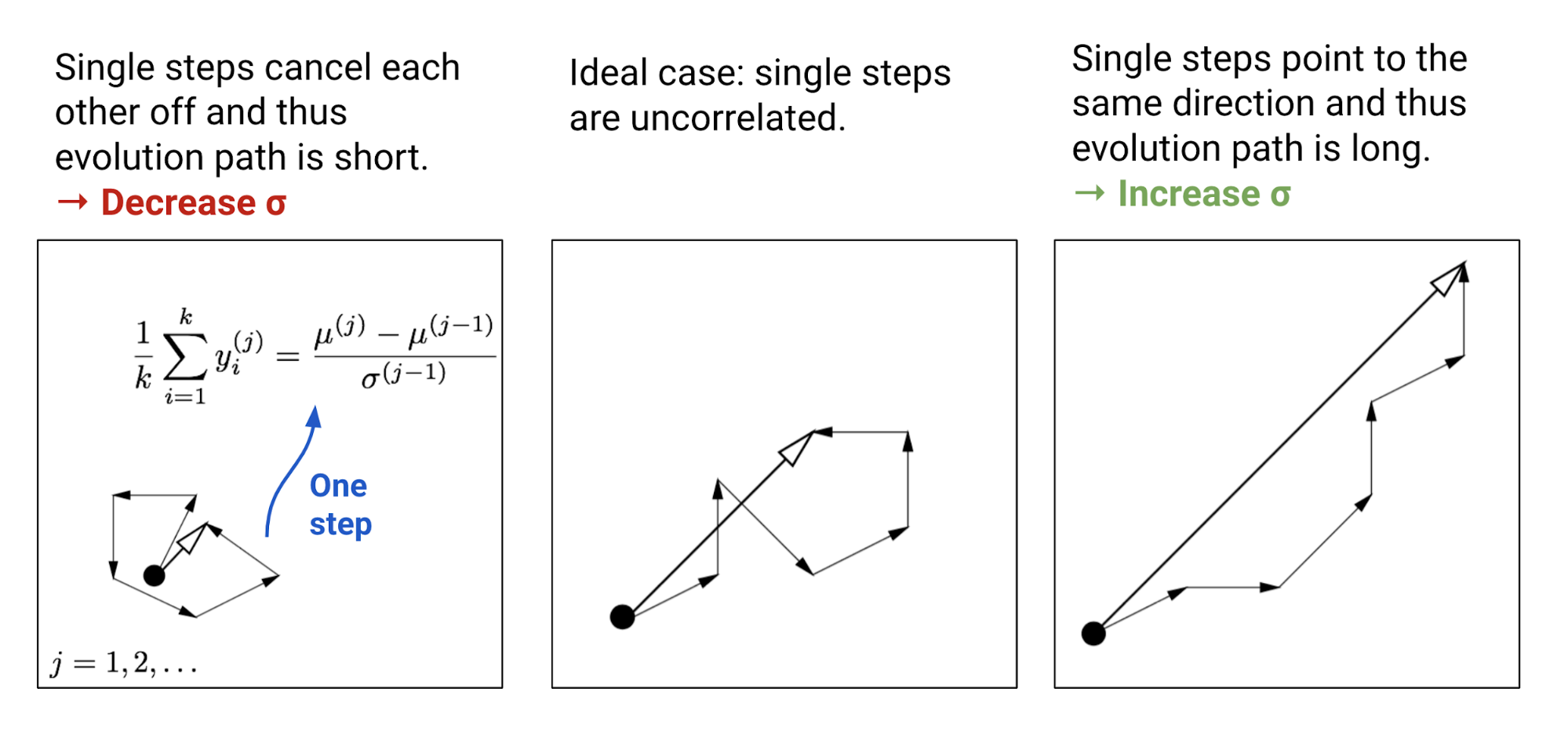
The parameter $\sigma$ controls the overall scale of the distribution. It is separated from the covariance matrix so that we can change steps faster than the full covariance. A larger step size leads to faster parameter update. In order to evaluate whether the current step size is proper, CMA-ES constructs an evolution path $p_\sigma$ by summing up a consecutive sequence of moving steps, $\frac{1}{\lambda}\sum_{i}^\lambda y_i^{(j)}, j=1, \dots, t$. By comparing this path length with its expected length under random selection (meaning single steps are uncorrelated), we are able to adjust $\sigma$ accordingly (See Fig. 2).
Each time the evolution path is updated with the average of moving step $y_i$ in the same generation.
By multiplying with $C^{-\frac{1}{2}}$, the evolution path is transformed to be independent of its direction. The term ${C^{(t)}}^{-\frac{1}{2}} = {B^{(t)}}^\top {D^{(t)}}^{-\frac{1}{2}} {B^{(t)}}$ transformation works as follows:
- ${B^{(t)}}$ contains row vectors of $C$’s eigenvectors. It projects the original space onto the perpendicular principal axes.
- Then ${D^{(t)}}^{-\frac{1}{2}} = \text{diag}(\frac{1}{\lambda_1}, \dots, \frac{1}{\lambda_n})$ scales the length of principal axes to be equal.
- ${B^{(t)}}^\top$ transforms the space back to the original coordinate system.
In order to assign higher weights to recent generations, we use polyak averaging to update the evolution path with learning rate $\alpha_\sigma$. Meanwhile, the weights are balanced so that $p_\sigma$ is conjugate, $\sim \mathcal{N}(0, I)$ both before and after one update.
The expected length of $p_\sigma$ under random selection is $\mathbb{E}|\mathcal{N}(0,I)|$, that is the expectation of the L2-norm of a $\mathcal{N}(0,I)$ random variable. Following the idea in Fig. 2, we adjust the step size according to the ratio of $|p_\sigma^{(t+1)}| / \mathbb{E}|\mathcal{N}(0,I)|$:
where $d_\sigma \approx 1$ is a damping parameter, scaling how fast $\ln\sigma$ should be changed.
Adapting the Covariance Matrix
For the covariance matrix, it can be estimated from scratch using $y_i$ of elite samples (recall that $y_i \sim \mathcal{N}(0, C)$):
The above estimation is only reliable when the selected population is large enough. However, we do want to run fast iteration with a small population of samples in each generation. That’s why CMA-ES invented a more reliable but also more complicated way to update $C$. It involves two independent routes,
- Rank-min(λ, n) update: uses the history of $\{C_\lambda\}$, each estimated from scratch in one generation.
- Rank-one update: estimates the moving steps $y_i$ and the sign information from the history.
The first route considers the estimation of $C$ from the entire history of $\{C_\lambda\}$. For example, if we have experienced a large number of generations, $C^{(t+1)} \approx \text{avg}(C_\lambda^{(i)}; i=1,\dots,t)$ would be a good estimator. Similar to $p_\sigma$, we also use polyak averaging with a learning rate to incorporate the history:
A common choice for the learning rate is $\alpha_{c\lambda} \approx \min(1, \lambda/n^2)$.
The second route tries to solve the issue that $y_i{y_i}^\top = (-y_i)(-y_i)^\top$ loses the sign information. Similar to how we adjust the step size $\sigma$, an evolution path $p_c$ is used to track the sign information and it is constructed in a way that $p_c$ is conjugate, $\sim \mathcal{N}(0, C)$ both before and after a new generation.
We may consider $p_c$ as another way to compute $\text{avg}_i(y_i)$ (notice that both $\sim \mathcal{N}(0, C)$) while the entire history is used and the sign information is maintained. Note that we’ve known $\sqrt{k}\frac{\mu^{(t+1)} - \mu^{(t)}}{\sigma^{(t)}} \sim \mathcal{N}(0, C)$ in the last section,
Then the covariance matrix is updated according to $p_c$:
The rank-one update approach is claimed to generate a significant improvement over the rank-min(λ, n)-update when $k$ is small, because the signs of moving steps and correlations between consecutive steps are all utilized and passed down through generations.
Eventually we combine two approaches together,
In all my examples above, each elite sample is considered to contribute an equal amount of weights, $1/\lambda$. The process can be easily extended to the case where selected samples are assigned with different weights, $w_1, \dots, w_\lambda$, according to their performances. See more detail in tutorial.
Natural Evolution Strategies
Natural Evolution Strategies (NES; Wierstra, et al, 2008) optimizes in a search distribution of parameters and moves the distribution in the direction of high fitness indicated by the natural gradient.
Natural Gradients
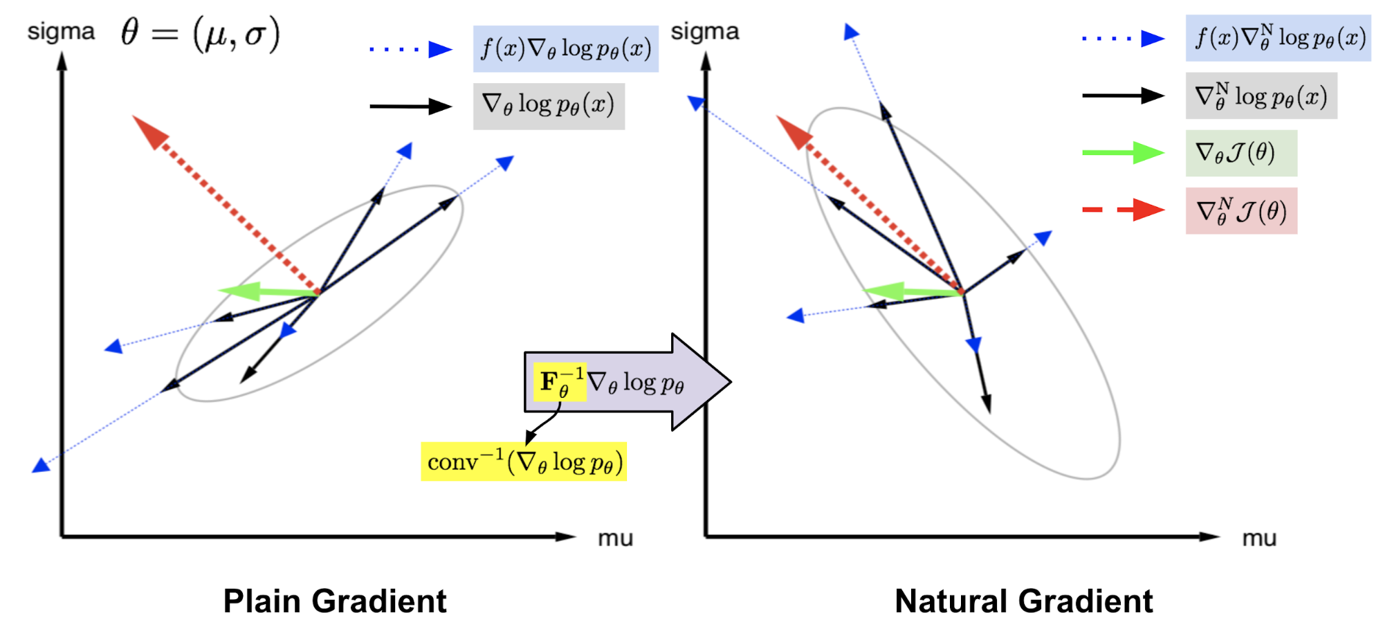
Given an objective function $\mathcal{J}(\theta)$ parameterized by $\theta$, let’s say our goal is to find the optimal $\theta$ to maximize the objective function value. A plain gradient finds the steepest direction within a small Euclidean distance from the current $\theta$; the distance restriction is applied on the parameter space. In other words, we compute the plain gradient with respect to a small change of the absolute value of $\theta$. The optimal step is:
Differently, natural gradient works with a probability distribution space parameterized by $\theta$, $p_\theta(x)$ (referred to as “search distribution” in NES paper). It looks for the steepest direction within a small step in the distribution space where the distance is measured by KL divergence. With this constraint we ensure that each update is moving along the distributional manifold with constant speed, without being slowed down by its curvature.
Estimation using Fisher Information Matrix
But, how to compute $\text{KL}[p_\theta | p_{\theta+\Delta\theta}]$ precisely? By running Taylor expansion of $\log p_{\theta + d}$ at $\theta$, we get:
where
Finally we have,
where $\mathbf{F}_\theta$ is called the Fisher Information Matrix and it is the covariance matrix of $\nabla_\theta \log p_\theta$ since $\mathbb{E}[\nabla_\theta \log p_\theta] = 0$.
The solution to the following optimization problem:
can be found using a Lagrangian multiplier,
where $d_\text{N}^*$ only extracts the direction of the optimal moving step on $\theta$, ignoring the scalar $\beta^{-1}$.
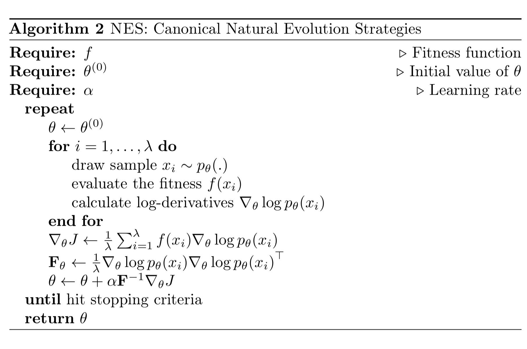
NES Algorithm
The fitness associated with one sample is labeled as $f(x)$ and the search distribution over $x$ is parameterized by $\theta$. NES is expected to optimize the parameter $\theta$ to achieve maximum expected fitness:
Using the same log-likelihood trick in REINFORCE:
Besides natural gradients, NES adopts a couple of important heuristics to make the algorithm performance more robust.
- NES applies rank-based fitness shaping, that is to use the rank under monotonically increasing fitness values instead of using $f(x)$ directly. Or it can be a function of the rank (“utility function”), which is considered as a free parameter of NES.
- NES adopts adaptation sampling to adjust hyperparameters at run time. When changing $\theta \to \theta’$, samples drawn from $p_\theta$ are compared with samples from $p_{\theta’}$ using [Mann-Whitney U-test(https://en.wikipedia.org/wiki/Mann%E2%80%93Whitney_U_test)]; if there shows a positive or negative sign, the target hyperparameter decreases or increases by a multiplication constant. Note the score of a sample $x’_i \sim p_{\theta’}(x)$ has importance sampling weights applied $w_i’ = p_\theta(x) / p_{\theta’}(x)$.
Applications: ES in Deep Reinforcement Learning
OpenAI ES for RL
The concept of using evolutionary algorithms in reinforcement learning can be traced back long ago, but only constrained to tabular RL due to computational limitations.
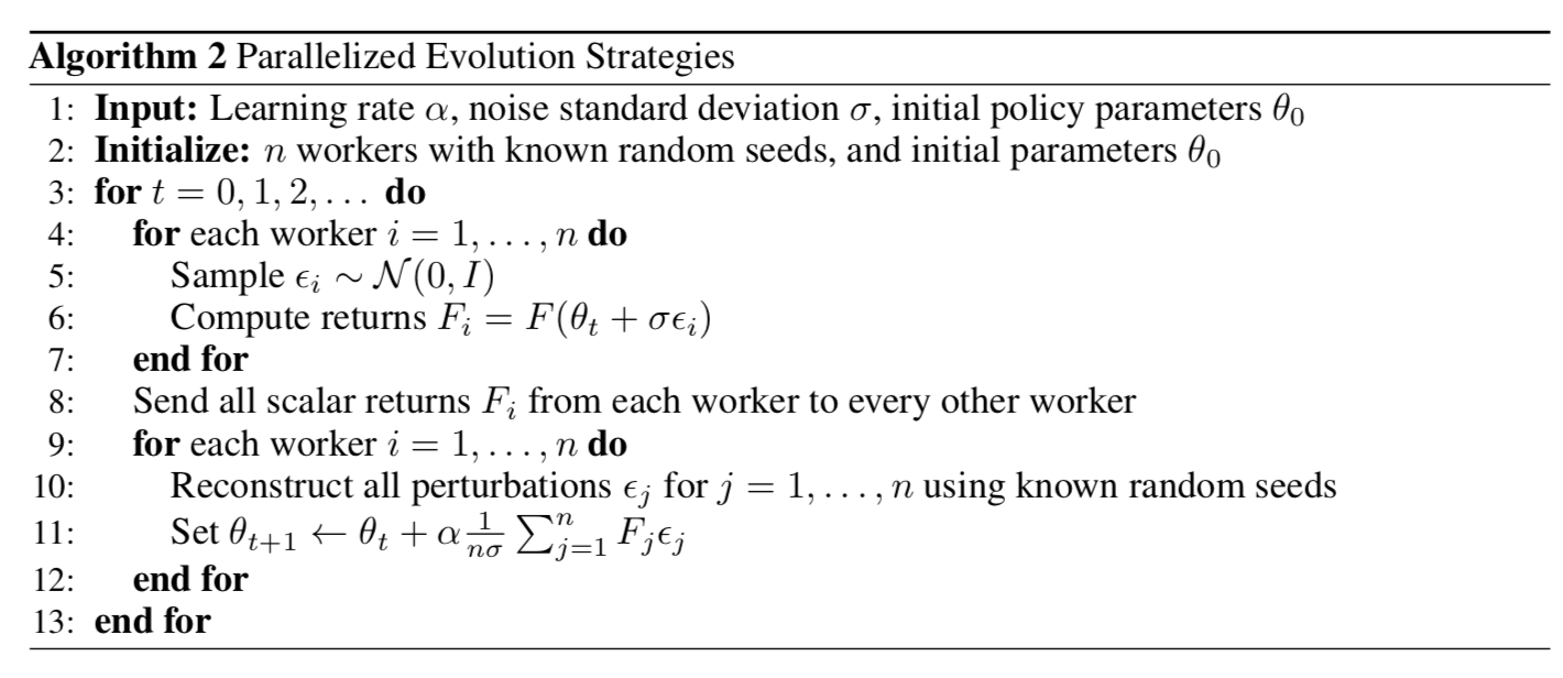
Inspired by NES, researchers at OpenAI (Salimans, et al. 2017) proposed to use NES as a gradient-free black-box optimizer to find optimal policy parameters $\theta$ that maximizes the return function $F(\theta)$. The key is to add Gaussian noise $\epsilon$ on the model parameter $\theta$ and then use the log-likelihood trick to write it as the gradient of the Gaussian pdf. Eventually only the noise term is left as a weighting scalar for measured performance.
Let’s say the current parameter value is $\hat{\theta}$ (the added hat is to distinguish the value from the random variable $\theta$). The search distribution of $\theta$ is designed to be an isotropic multivariate Gaussian with a mean $\hat{\theta}$ and a fixed covariance matrix $\sigma^2 I$,
The gradient for $\theta$ update is:
In one generation, we can sample many $epsilon_i, i=1,\dots,n$ and evaluate the fitness in parallel. One beautiful design is that no large model parameter needs to be shared. By only communicating the random seeds between workers, it is enough for the master node to do parameter update. This approach is later extended to adaptively learn a loss function; see my previous post on Evolved Policy Gradient.
To make the performance more robust, OpenAI ES adopts virtual batch normalization (BN with mini-batch used for calculating statistics fixed), mirror sampling (sampling a pair of $(-\epsilon, \epsilon)$ for evaluation), and fitness shaping.
Exploration with ES
Exploration (vs exploitation) is an important topic in RL. The optimization direction in the ES algorithm above is only extracted from the cumulative return $F(\theta)$. Without explicit exploration, the agent might get trapped in a local optimum.
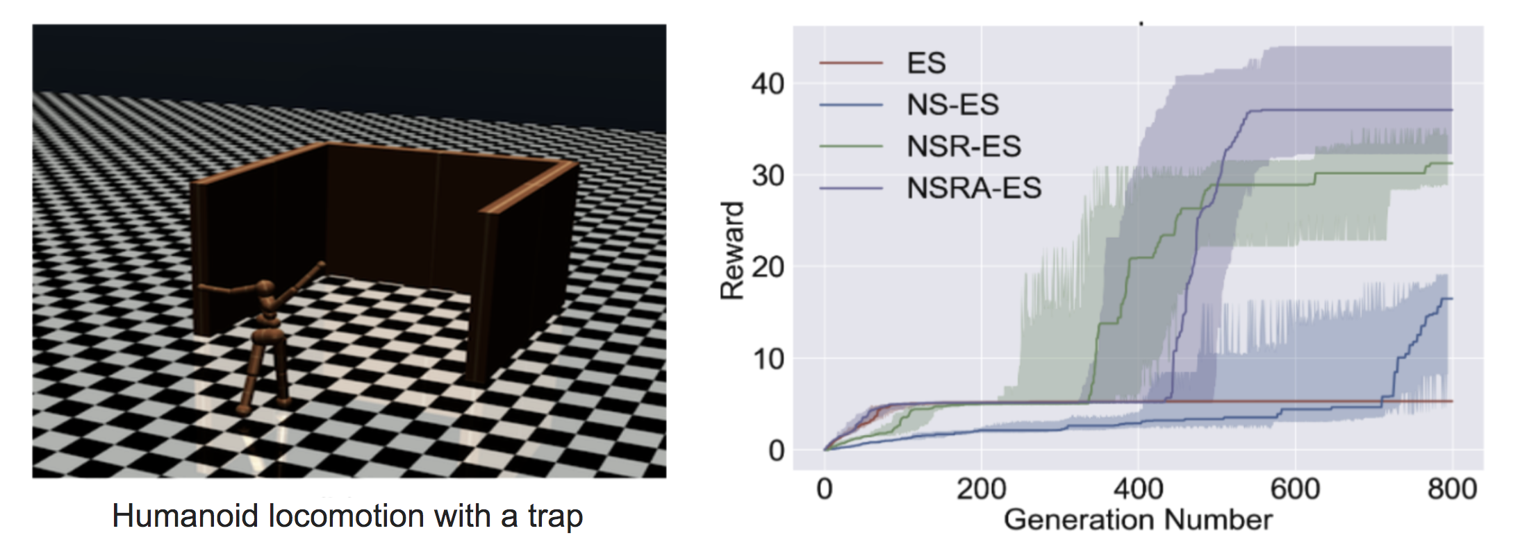
Novelty-Search ES (NS-ES; Conti et al, 2018) encourages exploration by updating the parameter in the direction to maximize the novelty score. The novelty score depends on a domain-specific behavior characterization function $b(\pi_\theta)$. The choice of $b(\pi_\theta)$ is specific to the task and seems to be a bit arbitrary; for example, in the Humanoid locomotion task in the paper, $b(\pi_\theta)$ is the final $(x,y)$ location of the agent.
- Every policy’s $b(\pi_\theta)$ is pushed to an archive set $\mathcal{A}$.
- Novelty of a policy $\pi_\theta$ is measured as the k-nearest neighbor score between $b(\pi_\theta)$ and all other entries in $\mathcal{A}$. (The use case of the archive set sounds quite similar to episodic memory.)
The ES optimization step relies on the novelty score instead of fitness:
NS-ES maintains a group of $M$ independently trained agents (“meta-population”), $\mathcal{M} = \{\theta_1, \dots, \theta_M \}$ and picks one to advance proportional to the novelty score. Eventually we select the best policy. This process is equivalent to ensembling; also see the same idea in SVPG.
where $N$ is the number of Gaussian perturbation noise vectors and $\alpha$ is the learning rate.
NS-ES completely discards the reward function and only optimizes for novelty to avoid deceptive local optima. To incorporate the fitness back into the formula, another two variations are proposed.
NSR-ES:
NSRAdapt-ES (NSRA-ES): the adaptive weighting parameter $w = 1.0$ initially. We start decreasing $w$ if performance stays flat for a number of generations. Then when the performance starts to increase, we stop decreasing $w$ but increase it instead. In this way, fitness is preferred when the performance stops growing but novelty is preferred otherwise.
CEM-RL
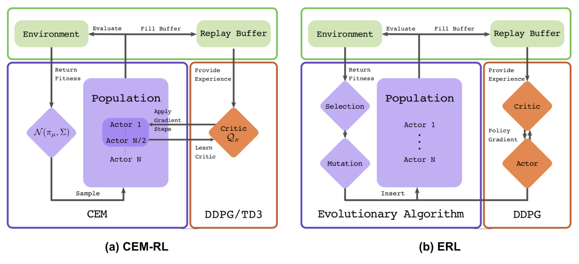
The CEM-RL method (Pourchot & Sigaud, 2019) combines Cross Entropy Method (CEM) with either DDPG or TD3. CEM here works pretty much the same as the simple Gaussian ES described above and therefore the same function can be replaced using CMA-ES. CEM-RL is built on the framework of Evolutionary Reinforcement Learning (ERL; Khadka & Tumer, 2018) in which the standard EA algorithm selects and evolves a population of actors and the rollout experience generated in the process is then added into reply buffer for training both RL-actor and RL-critic networks.
Workflow:
-
- The mean actor of the CEM population is $\pi_\mu$ is initialized with a random actor network.
-
- The critic network $Q$ is initialized too, which will be updated by DDPG/TD3.
-
- Repeat until happy:
- a. Sample a population of actors $\sim \mathcal{N}(\pi_\mu, \Sigma)$.
- b. Half of the population is evaluated. Their fitness scores are used as the cumulative reward $R$ and added into replay buffer.
- c. The other half are updated together with the critic.
- d. The new $\pi_mu$ and $\Sigma$ is computed using top performing elite samples. CMA-ES can be used for parameter update too.
Extension: EA in Deep Learning
(This section is not on evolution strategies, but still an interesting and relevant reading.)
The Evolutionary Algorithms have been applied on many deep learning problems. POET (Wang et al, 2019) is a framework based on EA and attempts to generate a variety of different tasks while the problems themselves are being solved. POET has been introduced in my last post on meta-RL. Evolutionary Reinforcement Learning (ERL) is another example; See Fig. 7 (b).
Below I would like to introduce two applications in more detail, Population-Based Training (PBT) and Weight-Agnostic Neural Networks (WANN).
Hyperparameter Tuning: PBT
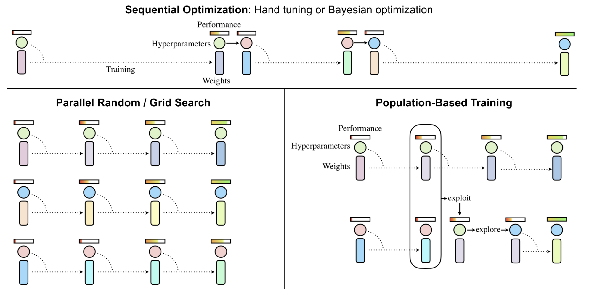
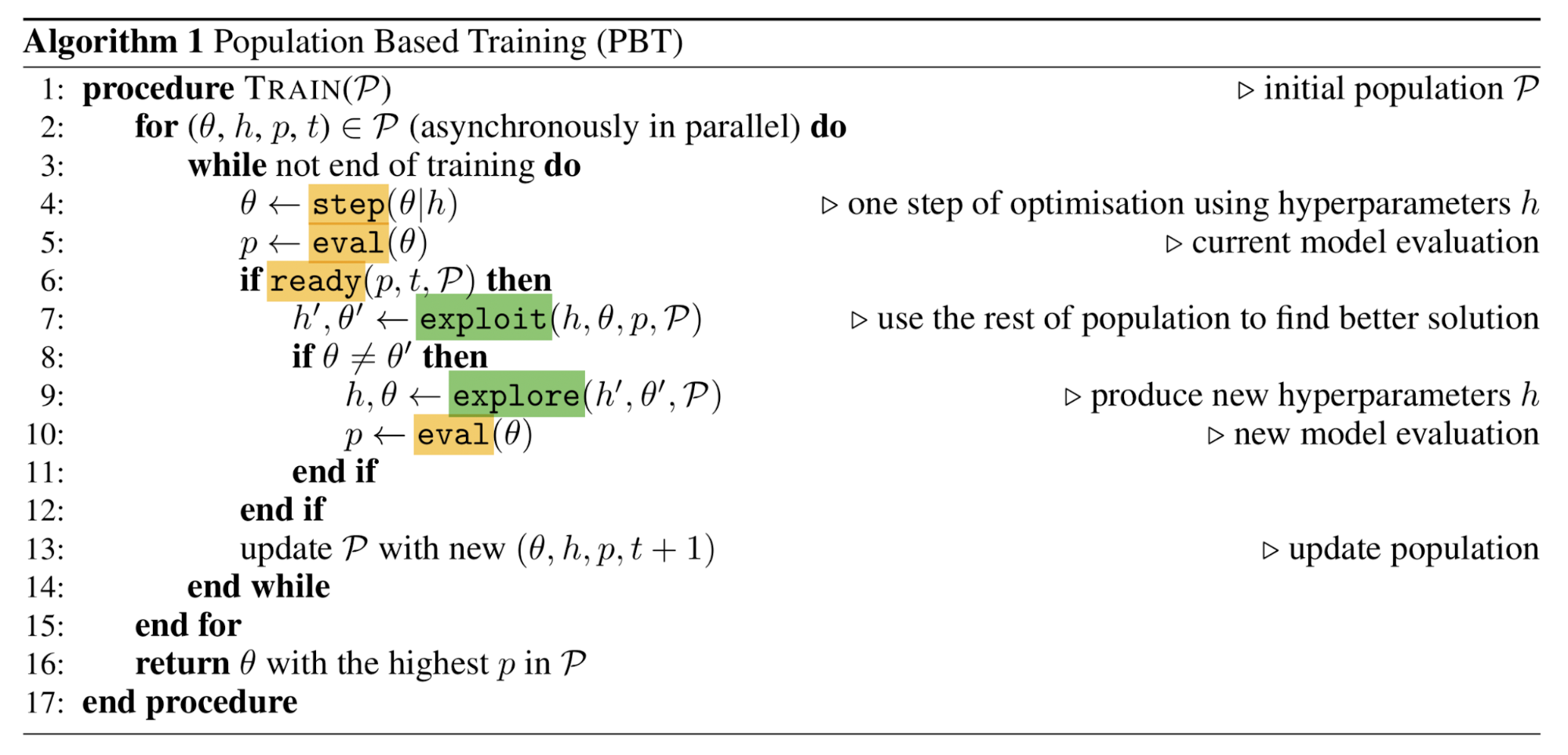
Population-Based Training (Jaderberg, et al, 2017), short for PBT applies EA on the problem of hyperparameter tuning. It jointly trains a population of models and corresponding hyperparameters for optimal performance.
PBT starts with a set of random candidates, each containing a pair of model weights initialization and hyperparameters, $\{(\theta_i, h_i)\mid i=1, \dots, N\}$. Every sample is trained in parallel and asynchronously evaluates its own performance periodically. Whenever a member deems ready (i.e. after taking enough gradient update steps, or when the performance is good enough), it has a chance to be updated by comparing with the whole population:
exploit(): When this model is under-performing, the weights could be replaced with a better performing model.explore(): If the model weights are overwritten,explorestep perturbs the hyperparameters with random noise.
In this process, only promising model and hyperparameter pairs can survive and keep on evolving, achieving better utilization of computational resources.
Network Topology Optimization: WANN
Weight Agnostic Neural Networks (short for WANN; Gaier & Ha 2019) experiments with searching for the smallest network topologies that can achieve the optimal performance without training the network weights. By not considering the best configuration of network weights, WANN puts much more emphasis on the architecture itself, making the focus different from NAS. WANN is heavily inspired by a classic genetic algorithm to evolve network topologies, called NEAT (“Neuroevolution of Augmenting Topologies”; Stanley & Miikkulainen 2002).
The workflow of WANN looks pretty much the same as standard GA:
- Initialize: Create a population of minimal networks.
- Evaluation: Test with a range of shared weight values.
- Rank and Selection: Rank by performance and complexity.
- Mutation: Create new population by varying best networks.
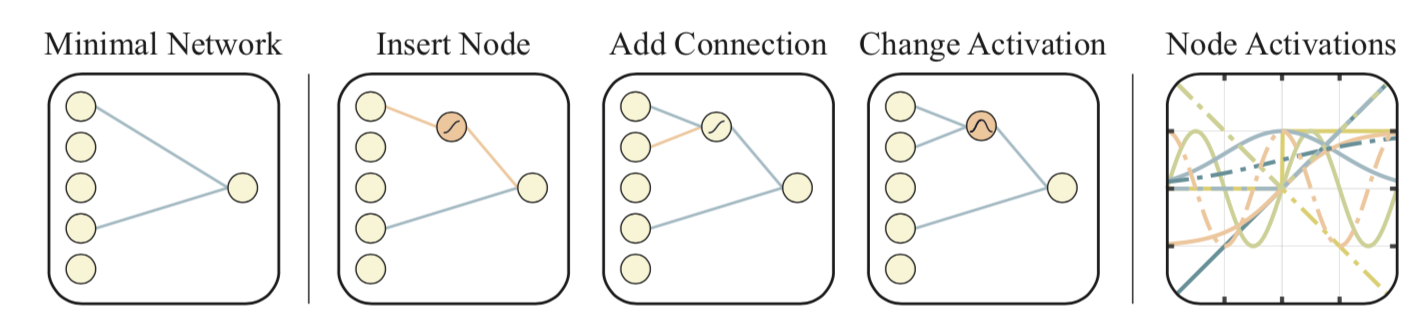
At the “evaluation” stage, all the network weights are set to be the same. In this way, WANN is actually searching for network that can be described with a minimal description length. In the “selection” stage, both the network connection and the model performance are considered.
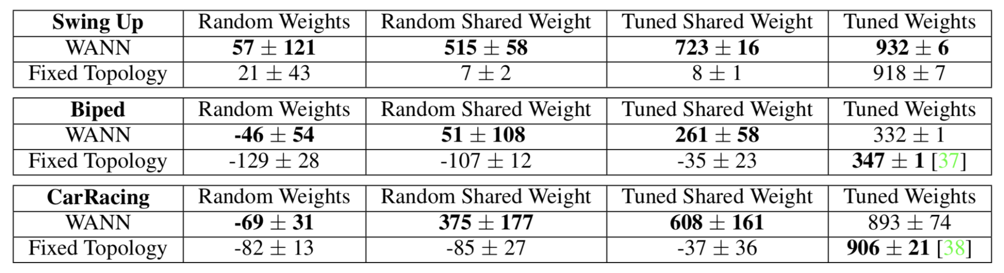
As shown in Fig. 11, WANN results are evaluated with both random weights and shared weights (single weight). It is interesting that even when enforcing weight-sharing on all weights and tuning this single parameter, WANN can discover topologies that achieve non-trivial good performance.
Cited as:
@article{weng2019ES,
  title   = "Evolution Strategies",
  author  = "Weng, Lilian",
  journal = "lilianweng.github.io",
  year    = "2019",
  url     = "https://lilianweng.github.io/posts/2019-09-05-evolution-strategies/"
}
References
[1] Nikolaus Hansen. “The CMA Evolution Strategy: A Tutorial” arXiv preprint arXiv:1604.00772 (2016).
[2] Marc Toussaint. Slides: “Introduction to Optimization”
[3] David Ha. “A Visual Guide to Evolution Strategies” blog.otoro.net. Oct 2017.
[4] Daan Wierstra, et al. “Natural evolution strategies.” IEEE World Congress on Computational Intelligence, 2008.
[5] Agustinus Kristiadi. “Natural Gradient Descent” Mar 2018.
[6] Razvan Pascanu & Yoshua Bengio. “Revisiting Natural Gradient for Deep Networks.” arXiv preprint arXiv:1301.3584 (2013).
[7] Tim Salimans, et al. “Evolution strategies as a scalable alternative to reinforcement learning.” arXiv preprint arXiv:1703.03864 (2017).
[8] Edoardo Conti, et al. “Improving exploration in evolution strategies for deep reinforcement learning via a population of novelty-seeking agents.” NIPS. 2018.
[9] Aloïs Pourchot & Olivier Sigaud. “CEM-RL: Combining evolutionary and gradient-based methods for policy search.” ICLR 2019.
[10] Shauharda Khadka & Kagan Tumer. “Evolution-guided policy gradient in reinforcement learning.” NIPS 2018.
[11] Max Jaderberg, et al. “Population based training of neural networks.” arXiv preprint arXiv:1711.09846 (2017).
[12] Adam Gaier & David Ha. “Weight Agnostic Neural Networks.” arXiv preprint arXiv:1906.04358 (2019).