[Updated on 2020-11-12: add an example on closed-book factual QA using OpenAI API (beta).
A model that can answer any question with regard to factual knowledge can lead to many useful and practical applications, such as working as a chatbot or an AI assistant🤖. In this post, we will review several common approaches for building such an open-domain question answering system.
Disclaimers given so many papers in the wild:
- Assume we have access to a powerful pretrained language model.
- We do not cover how to use structured knowledge base (e.g. Freebase, WikiData) here.
- We only focus on a single-turn QA instead of a multi-turn conversation style QA.
- We mostly focus on QA models that contain neural networks, specially Transformer-based language models.
- I admit that I missed a lot of papers with architectures designed specifically for QA tasks between 2017-2019😔
What is Open-Domain Question Answering?
Open-domain Question Answering (ODQA) is a type of language tasks, asking a model to produce answers to factoid questions in natural language. The true answer is objective, so it is simple to evaluate model performance.
For example,
Question: What did Albert Einstein win the Nobel Prize for?
Answer: The law of the photoelectric effect.
The “open-domain” part refers to the lack of the relevant context for any arbitrarily asked factual question. In the above case, the model only takes as the input the question but no article about “why Einstein didn’t win a Nobel Prize for the theory of relativity” is provided, where the term “the law of the photoelectric effect” is likely mentioned. In the case when both the question and the context are provided, the task is known as Reading comprehension (RC).
An ODQA model may work with or without access to an external source of knowledge (e.g. Wikipedia) and these two conditions are referred to as open-book or closed-book question answering, respectively.
When considering different types of open-domain questions, I like the classification by Lewis, et al., 2020, in increasing order of difficulty:
- A model is able to correctly memorize and respond with the answer to a question that has been seen at training time.
- A model is able to answer novel questions at test time and choose an answer from the set of answers it has seen during training.
- A model is able to answer novel questions which have answers not contained in the training dataset.
Notation
Given a question $x$ and a ground truth answer span $y$, the context passage containing the true answer is labelled as $z \in \mathcal{Z}$, where $\mathcal{Z}$ is an external knowledge corpus. Wikipedia is a common choice for such an external knowledge source.
Concerns of QA data fine-tuning
Before we dive into the details of many models below. I would like to point out one concern of fine-tuning a model with common QA datasets, which appears as one fine-tuning step in several ODQA models. It could be concerning, because there is a significant overlap between questions in the train and test sets in several public QA datasets.
Lewis, et al., (2020) (code) found that 58-71% of test-time answers are also present somewhere in the training sets and 28-34% of test-set questions have a near-duplicate paraphrase in their corresponding training sets. In their experiments, several models performed notably worse when duplicated or paraphrased questions were removed from the training set.
Open-book QA: Retriever-Reader
Given a factoid question, if a language model has no context or is not big enough to memorize the context which exists in the training dataset, it is unlikely to guess the correct answer. In an open-book exam, students are allowed to refer to external resources like notes and books while answering test questions. Similarly, a ODQA system can be paired with a rich knowledge base to identify relevant documents as evidence of answers.
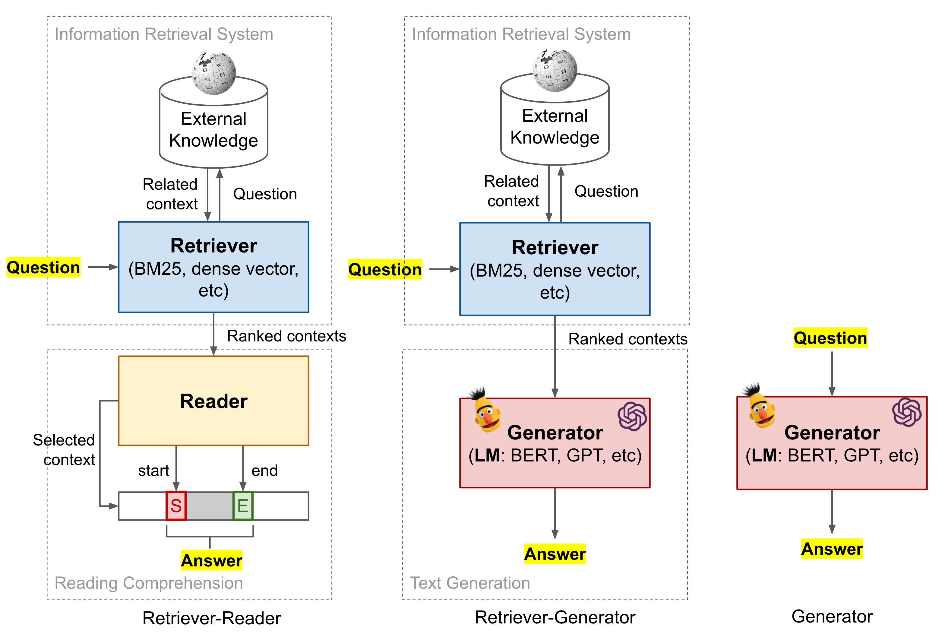
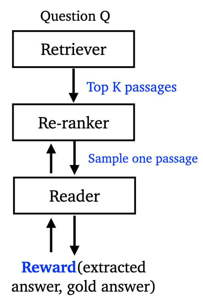
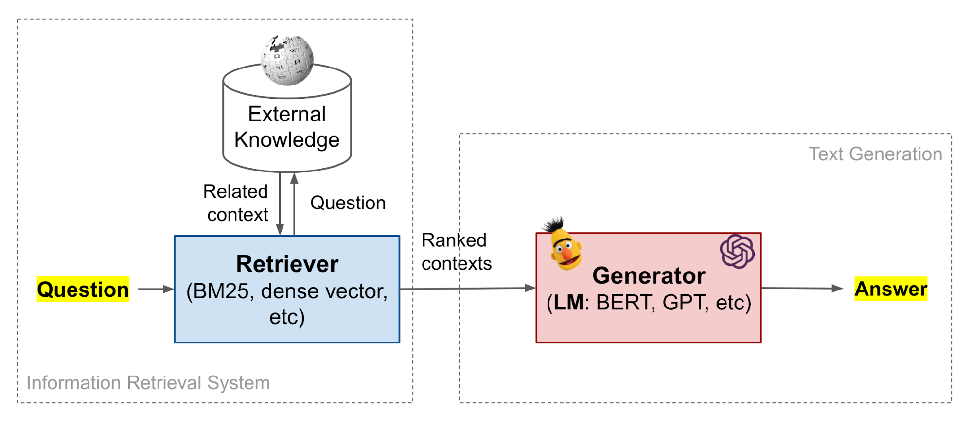
We can decompose the process of finding answers to given questions into two stages,
- Find the related context in an external repository of knowledge;
- Process the retrieved context to extract an answer.
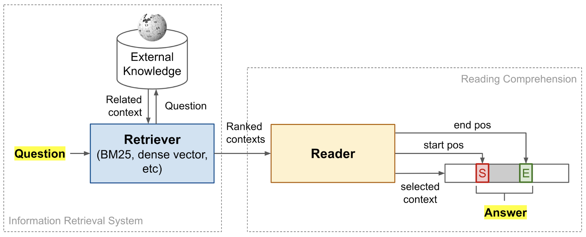
Such a retriever + reader framework was first proposed in DrQA (“Document retriever Question-Answering” by Chen et al., 2017; code). The retriever and the reader components can be set up and trained independently, or jointly trained end-to-end.
Retriever Model
Two popular approaches for implementing the retriever is to use the information retrieval (IR) system that depends on (1) the classic non-learning-based TF-IDF features (“classic IR”) or (2) dense embedding vectors of text produced by neural networks (“neural IR”).
Classic IR
DrQA (Chen et al., 2017) adopts an efficient non-learning-based search engine based on the vector space model. Every query and document is modelled as a bag-of-word vector, where each term is weighted by TF-IDF (term frequency $\times$ inverse document frequency).
where $t$ is a unigram or bigram term in a document $d$ from a collection of documents $\mathcal{D}$ . $\text{freq}(t, d)$ measures how many times a term $t$ appears in $d$. Note that the term-frequency here includes bigram counts too, which is found to be very helpful because the local word order is taken into consideration via bigrams. As part of the implementation, DrQA maps the bigrams of $2^{24}$ bins using unsigned murmur3 hash.
Precisely, DrQA implemented Wikipedia as its knowledge source and this choice has became a default setting for many ODQA studies since then. The non-ML document retriever returns the top $k=5$ most relevant Wikipedia articles given a question.
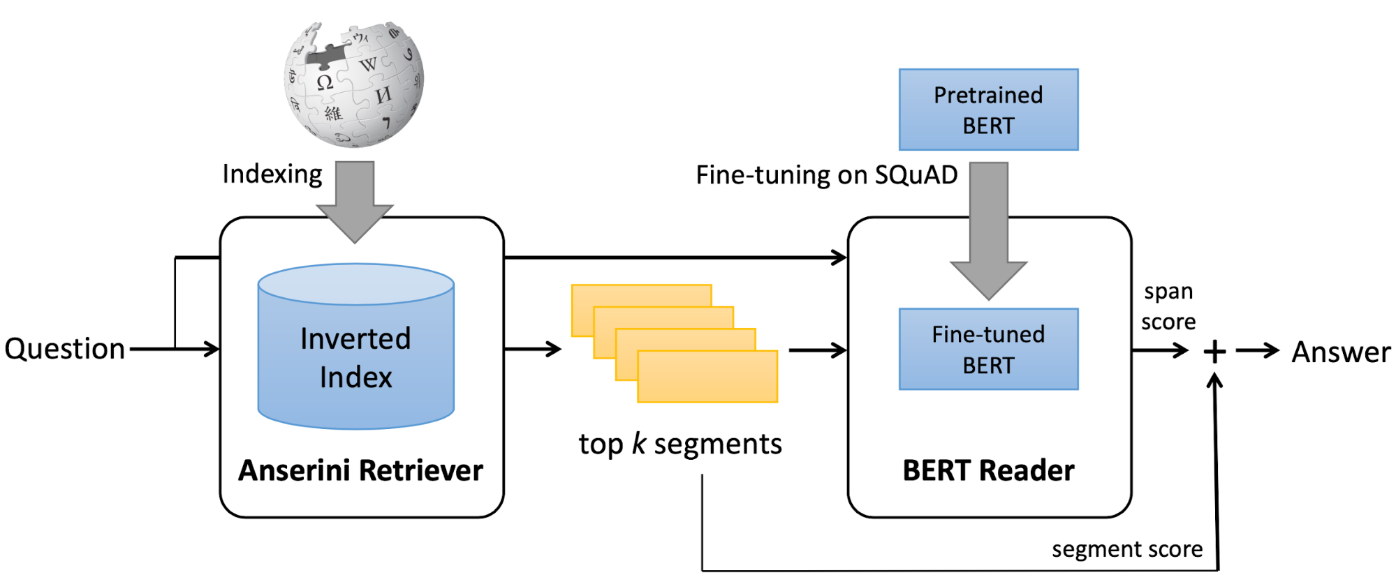
BERTserini (Yang et al., 2019) pairs the open-source Anserini IR toolkit as the retriever with a fine-tuned pre-trained BERT model as the reader. The top $k$ documents ($k=10$) are retrieved via the post-v3.0 branch of Anserini with the query treated as a bag of words. The retrieved text segments are ranked by BM25, a classic TF-IDF-based retrieval scoring function. In terms of the effect of text granularity on performance, they found that paragraph retrieval > sentence retrieval > article retrieval.
ElasticSearch + BM25 is used by the Multi-passage BERT QA model (Wang et al., 2019). They found that splitting articles into passages with the length of 100 words by sliding window brings 4% improvements, since splitting documents into passages without overlap may cause some near-boundary evidence to lose useful contexts.
Neural IR
There is a long history in learning a low-dimensional representation of text, denser than raw term-based vectors (Deerwester et al., 1990; Yih, et al., 2011). Dense representations can be learned through matrix decomposition or some neural network architectures (e.g. MLP, LSTM, bidirectional LSTM, etc). When involving neural networks, such approaches are referred to as “Neural IR”, Neural IR is a new category of methods for retrieval problems, but it is not necessary to perform better/superior than classic IR (Lim, 2018).
After the success of many large-scale general language models, many QA models embrace the following approach:
- Extract the dense representations of a question $x$ and a context passage $z$ by feeding them into a language model;
- Use the dot-product of these two representations as the retrieval score to rank and select most relevant passages.
ORQA, REALM and DPR all use such a scoring function for context retrieval, which will be described in detail in a later section on the end-to-end QA model.
An extreme approach, investigated by DenSPI (“Dense-Sparse Phrase Index”; Seo et al., 2019), is to encode all the text in the knowledge corpus at the phrase level and then only rely on the retriever to identify the most relevant phrase as the predicted answer. In this way, the retriever+reader pipeline is reduced to only retriever. Of course, the index would be much larger and the retrieval problem is more challenging.
DenSPI introduces a query-agnostic indexable representation of document phrases. Precisely it encodes query-agnostic representations of text spans in Wikipedia offline and looks for the answer at inference time by performing nearest neighbor search. It can drastically speed up the inference time, because there is no need to re-encode documents for every new query, which is often required by a reader model.
Given a question $x$ and a fixed set of (Wikipedia) documents, $z_1, \dots, z_K$ and each document $z_k$ contains $N_k$ words, $z_k = \langle z_k^{(1)}, \dots, z_k^{(N_k)}\rangle$. An ODQA model is a scoring function $F$ for each candidate phrase span $z_k^{(i:j)}, 1 \leq i \leq j \leq N_k$, such that the truth answer is the phrase with maximum score: $y = {\arg\max}_{k,i,j} F(x, z_k^{(i:j)})$.
The phrase representation $z_k^{(i:j)}$ combines both dense and sparse vectors, $z_k^{(i:j)} = [d_k^{(i:j)}, s_k^{(i:j)}] \in \mathbb{R}^{d^d + d^s}$ (note that $d^d \ll d^s$):
- The dense vector $d_k^{(i:j)}$ is effective for encoding local syntactic and semantic cues, as what can be learned by a pretrained language model.
- The sparse vector $s_k^{(i:j)}$ is superior at encoding precise lexical information. The sparse vector is term-frequency-based encoding. DenSPI uses 2-gram term-frequency same as DrQA, resulting a highly sparse representation ($d^s \approx 16$M)
The dense vector $d^{(i:j)}$ is further decomposed into three parts, $d^{(i:j)} = [a_i, b_j, c_{ij}] \in \mathbb{R}^{2d^b + 1}$ where $2d^b + 1 = d^d$. All three components are learned based on different columns of the fine-tuned BERT representations.
- A vector $a_i$ encodes the start position for the $i$-th word of the document;
- A vector $b_j$ encodes the end position for the $j$-th word of the document;
- A scalar $c_{ij}$ measures the coherency between the start and the end vectors, helping avoid non-constituent phrases during inference.
For all possible $(i,j,k)$ tuples where $j-i < J$, the text span embeddings are precomputed and stored as a phrase index. The maximum span length $J$ is a predefined scalar constant.
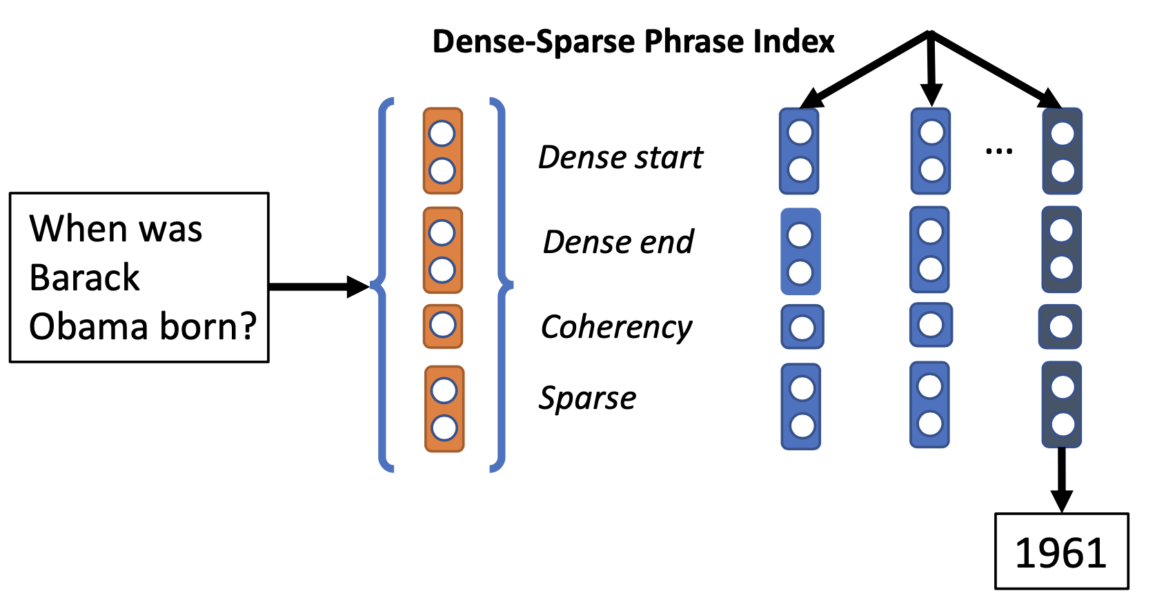
At the inference time, the question is mapped into the same vector space $x=[d’, s’] \in \mathbb{R}^{d^d + d^s}$, where the dense vector $d’$ is extracted from the BERT embedding of the special [CLS] symbol. The same BERT model is shared for encoding both questions and phrases. The final answer is predicted by $k^*, i^*, j^* = \arg\max x^\top z_k^{(i:j)}$.
Reader Model
The reader model learns to solve the reading comprehension task — extract an answer for a given question from a given context document. Here we only discuss approaches for machine comprehension using neural networks.
Bi-directional LSTM
The reader model for answer detection of DrQA (Chen et al., 2017) is a 3-layer bidirectional LSTM with hidden size 128. Every relevant paragraph of retrieved Wikipedia articles is encoded by a sequence of feature vector, $\{\tilde{\mathbf{z}}_1, \dots, \tilde{\mathbf{z}}_m \}$. Each feature vector $\hat{\mathbf{z}}_i \in \mathbb{R}^{d_z}$ is expected to capture useful contextual information around one token $z_i$. The feature consists of several categories of features:
- Word embeddings: A 300d Glove word embedding trained from 800B Web crawl data, $f_\text{embed} = E_g(z_i)$.
- Exact match: Whether a word $z_i$ appears in the question $x$, $f_\text{match} = \mathbb{I}(z_i \in x)$.
- Token features: This includes POS (part-of-speech) tagging, NER (named entity recognition), and TF (term-frequency), $f_\text{token}(z_i) = (\text{POS}(z_i), \text{NER}(z_i), \text{TF}(z_i))$.
- Aligned question embedding: The attention score $y_{ij}$ is designed to capture inter-sentence matching and similarity between the paragraph token $z_i$ and the question word $x_j$. This feature adds soft alignments between similar but non-identical words.
where $\alpha$ is a single dense layer with ReLU and $E_g(.)$ is the glove word embedding.
The feature vector of a paragraph of $m$ tokens is fed into LSTM to obtain the final paragraph vectors:
The question is encoded as a weighted sum of the embeddings of every word in the question:
where $\mathbf{w}$ is a weight vector to learn.
Once the feature vectors are constructed for the question and all the related paragraphs, the reader needs to predict the probabilities of each position in a paragraph to be the start and the end of an answer span, $p_\text{start}(i_s)$ and $p_\text{end}(i_s)$, respectively. Across all the paragraphs, the optimal span is returned as the final answer with maximum $p_\text{start}(i_s) \times p_\text{end}(i_e) $.
where $\mathbf{W}_s$ and $\mathbf{W}_e$ are learned parameters.
BERT-universe
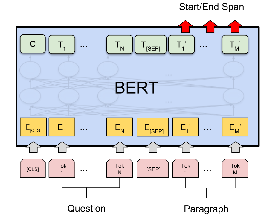
Following the success of BERT (Devlin et al., 2018), many QA models develop the machine comprehension component based on BERT. Let’s define the BERT model as a function that can take one or multiple strings (concatenated by [SEP]) as input and outputs a set of BERT encoding vectors for the special [CLS] token and every input token:
where $\mathbf{h}^\texttt{[CLS]}$ is the embedding vector for the special [CLS] token and $\mathbf{h}^{(i)}$ is the embedding vector for the $i$-th token.
To use BERT for reading comprehension, it learns two additional weights, $\mathbf{W}_s$ and $\mathbf{W}_e$, and $\text{softmax}(\mathbf{h}^{(i)}\mathbf{W}_s)$ and $\text{softmax}(\mathbf{h}^{(i)}\mathbf{W}_e)$ define two probability distributions of start and end position of the predicted span per token.
BERTserini (Yang et al., 2019) utilizes a pre-trained BERT model to work as the reader. Their experiments showed that fine-tuning pretrained BERT with SQuAD is sufficient to achieve high accuracy in identifying answer spans.
The key difference of the BERTserini reader from the original BERT is: to allow comparison and aggregation of results from different segments, the final softmax layer over different answer spans is removed. The pre-trained BERT model is fine-tuned on the training set of SQuAD, where all inputs to the reader are padded to 384 tokens with the learning rate 3e-5.
When ranking all the extracted answer spans, the retriever score (BM25) and the reader score (probability of token being the start position $\times$ probability of the same token being the end position ) are combined via linear interpolation.
The original BERT normalizes the probability distributions of start and end position per token for every passage independently. Differently, the Multi-passage BERT (Wang et al., 2019) normalizes answer scores across all the retrieved passages of one question globally. Precisely, multi-passage BERT removes the final normalization layer per passage in BERT for QA (same as in BERTserini) and then adds a global softmax over all the word positions of all the passages. Global normalization makes the reader model more stable while pin-pointing answers from a large number of passages.
In addition, multi-passage BERT implemented an independent passage ranker model via another BERT model and the rank score for $(x, z)$ is generated by a softmax over the representation vectors of the first [CLS] token. The passage ranker brings in extra 2% improvements. Similar idea of re-ranking passages with BERT was discussed in Nogueira & Cho, 2019, too.
Interestingly, Wang et al., 2019 found that explicit inter-sentence matching does not seem to be critical for RC tasks with BERT; check the original paper for how the experiments were designed. One possible reason is that the multi-head self-attention layers in BERT has already embedded the inter-sentence matching.
End-to-end Joint Training
The retriever and reader components can be jointly trained. This section covers R^3, ORQA, REALM and DPR. There are a lot of common designs, such as BERT-based dense vectors for retrieval and the loss function on maximizing the marginal likelihood of obtaining true answers.
The retriever and reader models in the R^3 (“Reinforced Ranker-Reader”; Wang, et al., 2017) QA system are jointly trained via reinforcement learning. (Note that to keep the term consistent between papers in this section, the “ranker” model in the original R^3 paper is referred to as the “retriever” model here.) Both components are variants of Match-LSTM, which relies on an attention mechanism to compute word similarities between the passage and question sequences.
How does the Match-LSTM module work? Given a question $\mathbf{X}$ of $d_x$ words and a passage $\mathbf{Z}$ of $d_z$ words, both representations use fixed Glove word embeddings,
where $l$ is the hidden dimension of the bidirectional LSTM module. $\mathbf{W}^g \in \mathbb{R}^{l\times l}$, $\mathbf{b}^g \in \mathbb{R}^l$, and $\mathbf{W}^m \in \mathbb{R}^{2l \times 4l}$ are parameters to learn. The operator $\otimes \mathbf{e}_{d_x}$ is the outer product to repeat the column vector $\mathbf{b}^g$ $d_x$ times.
The ranker and reader components share the same Match-LSTM module with two separate prediction heads in the last layer, resulting in $\mathbf{H}^\text{rank}$ and $\mathbf{H}^\text{reader}$.
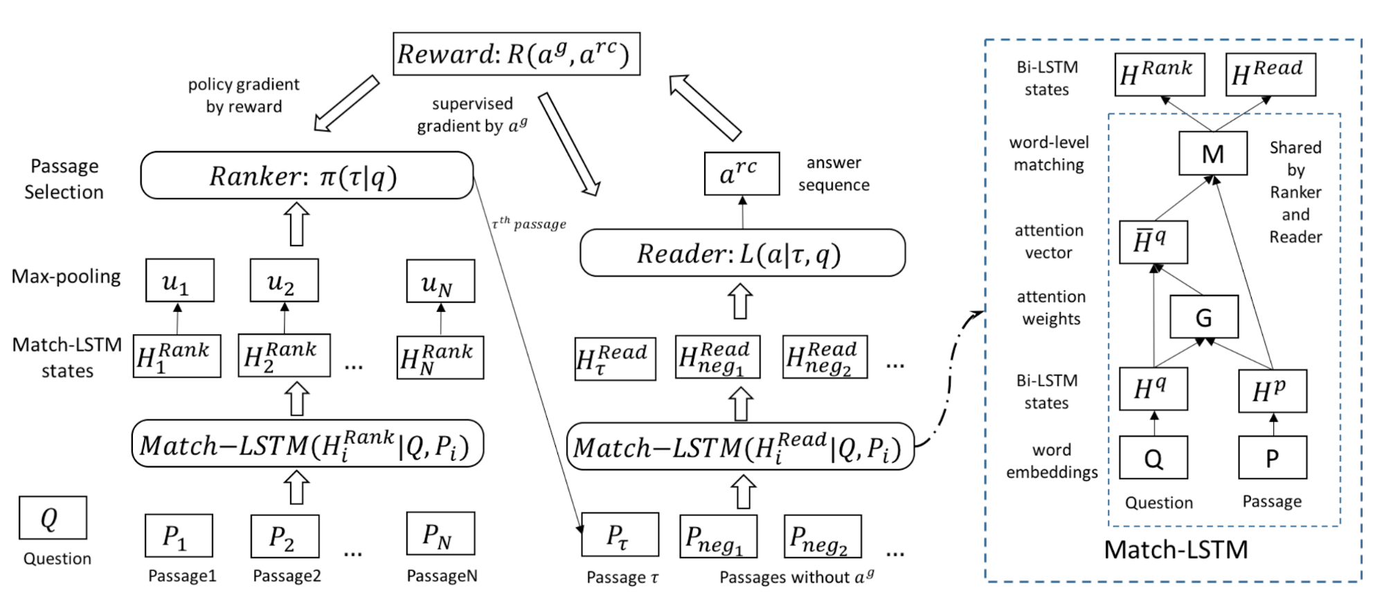
The retriever runs a max-pooling operation per passage and then aggregates to output a probability of each passage entailing the answer.
Finally, the retriever is viewed as a policy to output action to sample a passage according to predicted $\gamma$,
The reader predicts the start position $\beta^s$ and the end position $\beta^e$ of the answer span. Two positions are computed in the same way, with independent parameters to learn. There are $V$ words in all the passages involved.
where $y$ is the ground-truth answer and the passage $z$ is sampled by the retriever. $\beta^s_{y_z^s}$ and $\beta^s_{y_z^e}$ represent the probabilities of the start and end positions of $y$ in passage $z$.
The training objective for the end-to-end R^3 QA system is to minimize the negative log-likelihood of obtaining the correct answer $y$ given a question $x$,
Essentially in training, given a passage $z$ sampled by the retriever, the reader is trained by gradient descent while the retriever is trained by REINFORCE using $L(y \vert z, x)$ as the reward function. However, $L(y \vert z, x)$ is not bounded and may introduce a lot of variance. The paper replaces the reward with a customized scoring function by comparing the ground truth $y$ and the answer extracted by the reader $\hat{y}$:
ORQA (“Open-Retrieval Question-Answering”; Lee et al., 2019) jointly learns a retriever + reader QA model to optimize marginal log-likelihood of obtaining correct answers in a supervised manner. No explicit “black-box” IR system is involved. Instead, it is capable of retrieving any text in an open corpus. During training, ORQA does not need ground-truth context passages (i.e. reading comprehension datasets) but only needs (question, answer) string pairs. Both retriever and reader components are based on BERT, but not shared.
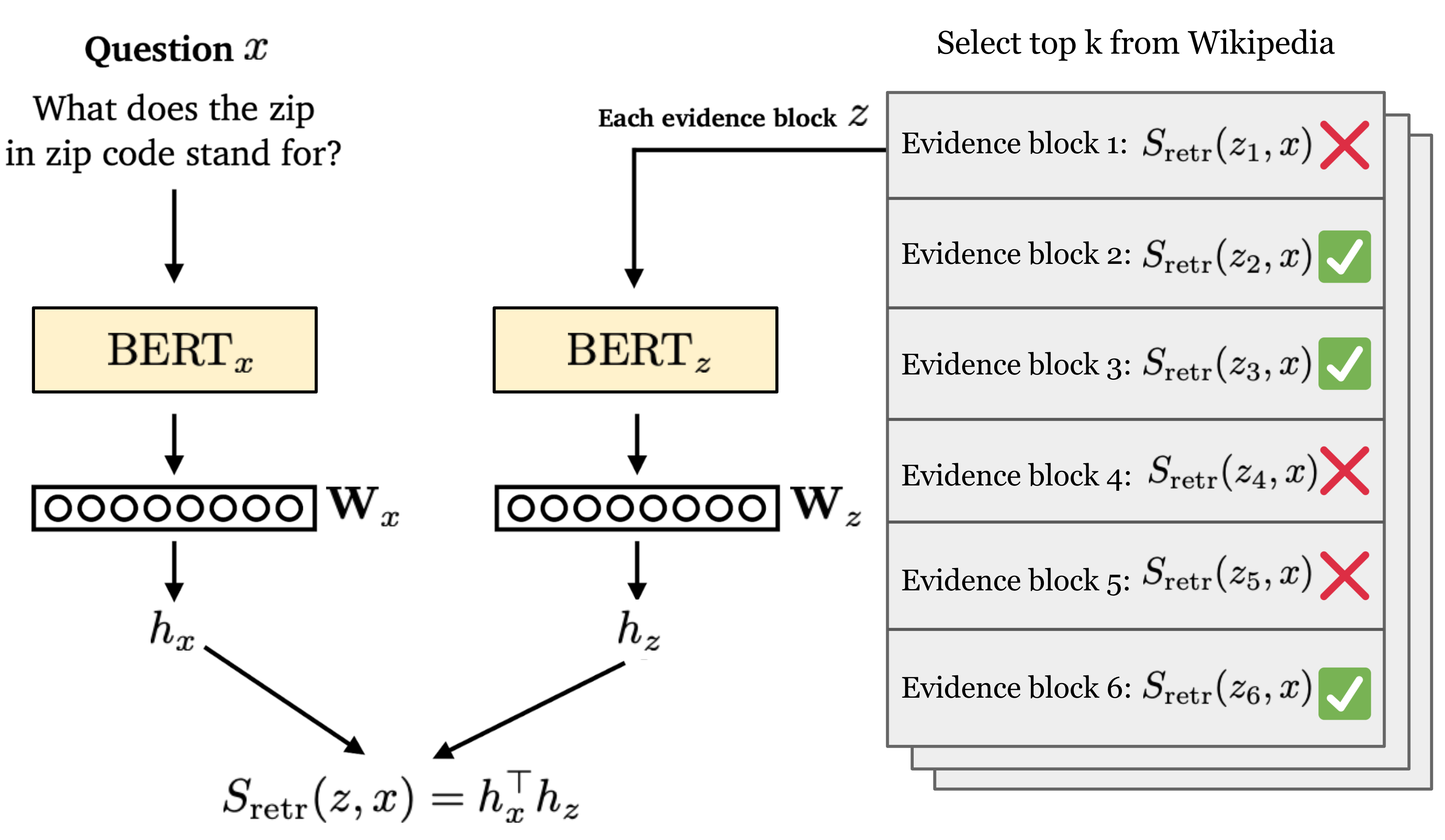
All the evidence blocks are ranked by a retrieval score, defined as the inner product of BERT embedding vectors of the [CLS] token of the question $x$ and the evidence block $z$. Note that the encoders for questions and context are independent.
The retriever module is pretrained with Inverse Cloze Task (ICT), which is to predict the context given a sentence, opposite to the standard Cloze Task. The ICT objective is to maximize the retrieval score of the correct context $z$ given a random sentence $x$:
where $\text{BATCH}(\mathcal{Z})$ is the set of evidence blocks in the same batch used as sampled negatives.
After such pretraining, the BERT retriever is expected to have representations good enough for evidence retrieval. Only the question encoder needs to be fine-tuned for answer extraction. In other words, the evidence block encoder (i.e., $\mathbf{W}_z$ and $\text{BERT}_z$) is fixed and thus all the evidence block encodings can be pre-computed with support for fast Maximum Inner Product Search (MIPS).
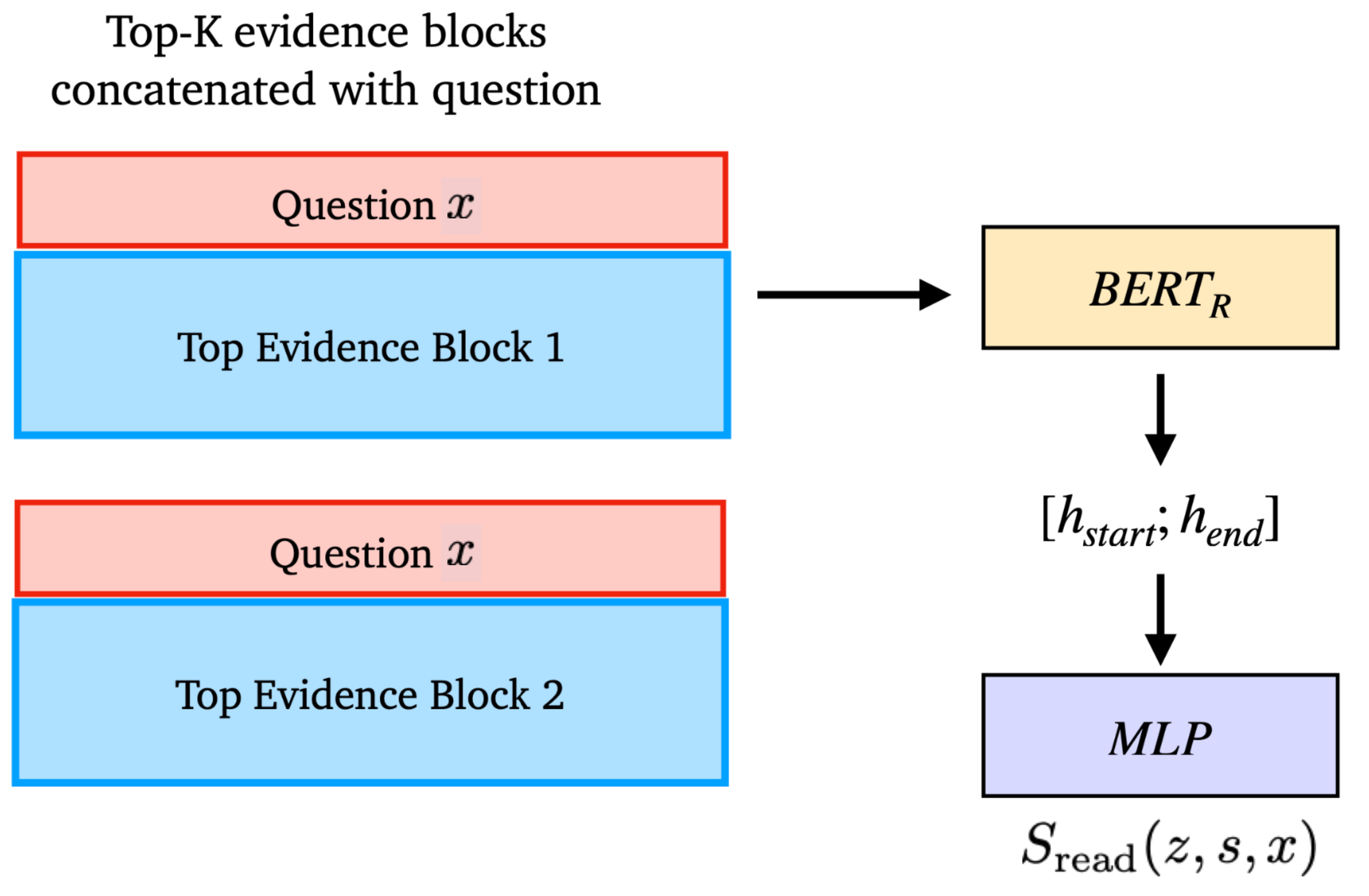
The reader follows the same design as in the original BERT RC experiments. It learns in a supervised manner, while the parameters of the evidence block encoder are fixed and all other parameters are fine-tuned. Given a question $x$ and a gold answer string $y$, the reader loss contains two parts:
(1) Find all correct text spans within top $k$ evidence blocks and optimize for the marginal likelihood of a text span $s$ that matches the true answer $y$:
where $y=\text{TEXT}(s)$ indicates whether the answer $y$ matches the text span $s$. $\text{TOP}(k)$ is the top $k$ retrieved blocks according to $S_\text{retr}(z, x)$. The paper sets $k=5$.
(2) At the early stage of learning, when the retriever is not strong enough, it is possible none of the top $k$ blocks contains the answer. To avoid such sparse learning signals, ORQA considers a larger set of $c$ evidence blocks for more aggressive learning. The paper has $c=5000$.
Some issues in SQuAD dataset were discussed in the ORQA paper:
" The notable drop between development and test accuracy for SQuAD is a reflection of an artifact in the dataset—its 100k questions are derived from only 536 documents. Therefore, good retrieval targets are highly correlated between training examples, violating the IID assumption, and making it unsuitable for learned retrieval. We strongly suggest that those who are interested in end-to-end open-domain QA models no longer train and evaluate with SQuAD for this reason."
REALM (“Retrieval-Augmented Language Model pre-training”; Guu et al., 2020) also jointly trains retriever + reader by optimizing the marginal likelihood of obtaining the true answer:
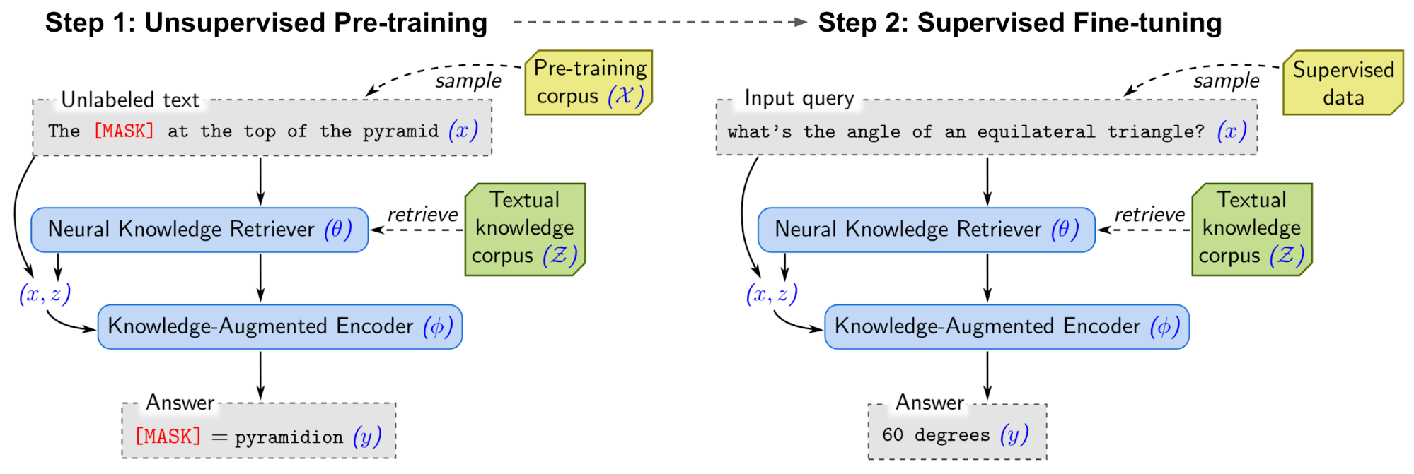
REALM computes two probabilities, $p(z \vert x)$ and $p(y \vert x, z)$, same as ORQA. However, different from ICT in ORQA, REALM upgrades the unsupervised pre-training step with several new design decisions, leading towards better retrievals. REALM pre-trains the model with Wikipedia or CC-News corpus.
- Use salient span masking. Named entities and dates are identified. Then one of these “salient spans” is selected and masked. Salient span masking is a special case of MLM and works out well for QA tasks.
- Add an empty null document. Because not every question demands a context document.
- No trivial retrieval. The context document should not be same as the selected sentence with a masked span.
- Apply the same ICT loss as in ORQA to encourage learning when the retrieval quality is still poor at the early stage of training.
“Among all systems, the most direct comparison with REALM is ORQA (Lee et al., 2019), where the fine-tuning setup, hyperparameters and training data are identical. The improvement of REALM over ORQA is purely due to better pre-training methods.” — from REALM paper.
Both unsupervised pre-training and supervised fine-tuning optimize the same log-likelihood $\log p(y \vert x)$. Because the parameters of the retriever encoder for evidence documents are also updated in the process, the index for MIPS is changing. REALM asynchronously refreshes the index with the updated encoder parameters every several hundred training steps.
Balachandran, et al. (2021) found that REALM is significantly undertrained and REALM++ achieves great EM accuracy improvement (3-5%) by scaling up the model training with larger batch size and more retrieved documents for the reader to process.
DPR (“Dense Passage Retriever”; Karpukhin et al., 2020, code) argues that ICT pre-training could be too computationally expensive and the ORQA’s context encoder might be sub-optimal because it is not fine-tuned with question-answer pairs. DPR aims to resolve these two issues by only training a dense dual-encoder architecture for retrieval only from a small number of Q/A pairs, without any pre-training.
Same as previous work, DPR uses the dot-product (L2 distance or cosine similarity also works) of BERT representations as retrieval score. The loss function for training the dual-encoder is the NLL of the positive passage, which essentially takes the same formulation as ICT loss of ORQA. Note that both of them consider other passages in the same batch as the negative samples, named in-batch negative sampling. The main difference is that DPR relies on supervised QA data, while ORQA trains with ICT on unsupervised corpus. At the inference time, DPR uses FAISS to run fast MIPS.
DPR did a set of comparison experiments involving several different types of negatives:
- Random: any random passage from the corpus;
- BM25: top passages returned by BM25 which don’t contain the answer but match most question tokens;
- In-batch negative sampling (“gold”): positive passages paired with other questions which appear in the training set.
DPR found that using gold passages from the same mini-batch and one negative passage with high BM25 score works the best. To further improve the retrieval results, DPR also explored a setting where a BM25 score and a dense embedding retrieval score are linearly combined to serve as a new ranking function.
Open-book QA: Retriever-Generator
Compared to the retriever-reader approach, the retriever-generator also has 2 stages but the second stage is to generate free text directly to answer the question rather than to extract start/end position in a retrieved passage. Some paper also refer to this as Generative question answering.
A pretrained LM has a great capacity of memorizing knowledge in its parameters, as shown above. However, they cannot easily modify or expand their memory, cannot straightforwardly provide insights into their predictions, and may produce non-existent illusion.
Petroni et al. (2020) studied how the retrieved relevant context can help a generative language model produce better answers. They found:
- Augmenting queries with relevant contexts dramatically improves the pretrained LM on unsupervised machine reading capabilities.
- An off-the-shelf IR system is sufficient for BERT to match the performance of a supervised ODQA baseline;
- BERT’s NSP pre-training strategy is a highly effective unsupervised mechanism in dealing with noisy and irrelevant contexts.
They pair the BERT model with different types of context, including adversarial (unrelated context), retrieved (by BM25), and generative (by an autoregressive language model of 1.4N parameters, trained on CC-NEWS). The model is found to be robust to adversarial context, but only when the question and the context are provided as two segments (e.g. separated by [SEP]). One hypothesis is related to NSP task: “BERT might learn to not condition across segments for masked token prediction if the NSP score is low, thereby implicitly detecting irrelevant and noisy contexts.”
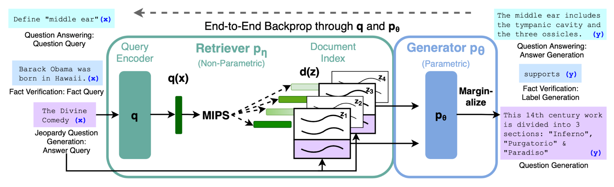
RAG (“Retrieval-Augmented Generation”; Lewis et al., 2020) combines pre-trained parametric (language model) and non-parametric memory (external knowledge index) together for language generation. RAG can be fine-tuned on any seq2seq task, whereby both the retriever and the sequence generator are jointly learned. They found that unconstrained generation outperforms previous extractive approaches.
RAG consists of a retriever model $p_\eta(z \vert x)$ and a generator model $p_\theta(y_i \vert x, z, y_{1:i-1})$:
- The retriever uses the input sequence $x$ to retrieve text passages $z$, implemented as a DPR retriever. $\log p_\eta(z \vert x) \propto E_z(z)^\top E_x(x)$.
- The generator uses $z$ as additional context when generating the target sequence $y$, where the context and the question are simply concatenated.
Depending on whether using the same or different retrieved documents for each token generation, there are two versions of RAG:
The retriever + generator in RAG is jointly trained to minimize the NLL loss, $\mathcal{L}_\text{RAG} = \sum_j -\log p(y_j \vert x_j)$. Updating the passage encoder $E_z(.)$ is expensive as it requires the model to re-index the documents for fast MIPS. RAG does not find fine-tuning $E_z(.)$ necessary (like in ORQA) and only updates the query encoder + generator.
At decoding/test time, RAG-token can be evaluated via a beam search. RAG-seq cannot be broken down into a set of per-token likelihood, so it runs beam search for each candidate document $z$ and picks the one with optimal $p_\theta(y_i \vert x, z, y_{1:i-1})$.
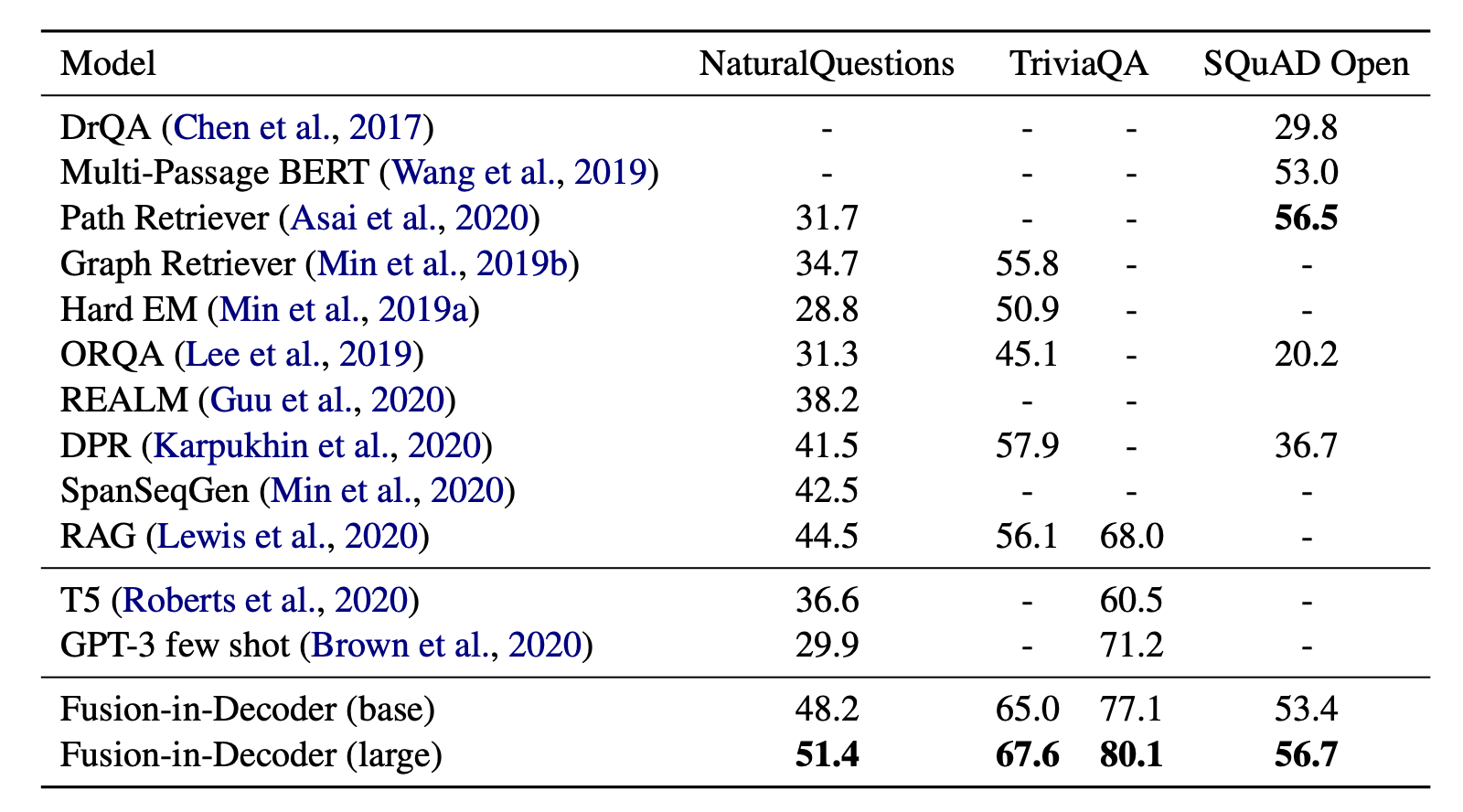
The Fusion-in-Decoder approach, proposed by Izacard & Grave (2020) is also based on a pre-trained T5. It works similar to RAG but differently for how the context is integrated into the decoder.
- Retrieve top $k$ related passage of 100 words each, using BM25 or DPR.
- Each retrieved passage and its title are concatenated with the question using special tokens like
question:,title:andcontext:to indicate the content differences. - Each retrieved passage is processed independently and later combined in the decoder. Processing passages independently in the encoder allows us to parallelize the computation. OTOH, processing them jointly encourages better aggregation of multiple pieces of evidence. The aggregation part is missing in extractive approaches.
Note that they did fine-tune the pretrained LM independently for each dataset.
Closed-book QA: Generative Language Model
Big language models have been pre-trained on a large collection of unsupervised textual corpus. Given enough parameters, these models are able to memorize some factual knowledge within parameter weights. Therefore, we can use these models to do question-answering without explicit context, just like in a closed-book exam. The pre-trained language models produce free text to respond to questions, no explicit reading comprehension.

Roberts et al. (2020) measured the practical utility of a language model by fine-tuning a pre-trained model to answer questions without access to any external context or knowledge. They fine-tuned the T5 language model (same architecture as the original Transformer) to answer questions without inputting any additional information or context. Such setup enforces the language model to answer questions based on “knowledge” that it internalized during pre-training.
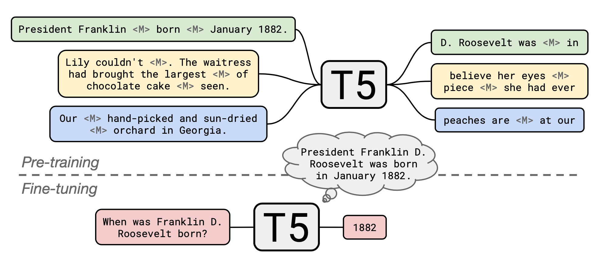
The original T5 models were pre-trained on a multi-task mixture including an unsupervised “masked language modeling” (MLM) tasks on the C4 (“Colossal Clean Crawled Corpus”) dataset as well as fine-tuned altogether with supervised translation, summarization, classification, and reading comprehension tasks. Roberts, et al. (2020) took a pre-trained T5 model and continued pre-training with salient span masking over Wikipedia corpus, which has been found to substantially boost the performance for ODQA. Then they fine-tuned the model for each QA datasets independently.
With a pre-trained T5 language model + continue pre-training with salient spans masking + fine-tuning for each QA dataset,
- It can attain competitive results in open-domain question answering without access to external knowledge.
- A larger model can obtain better performance. For example, a T5 with 11B parameters is able to match the performance with DPR with 3 BERT-base models, each with 330M parameters.
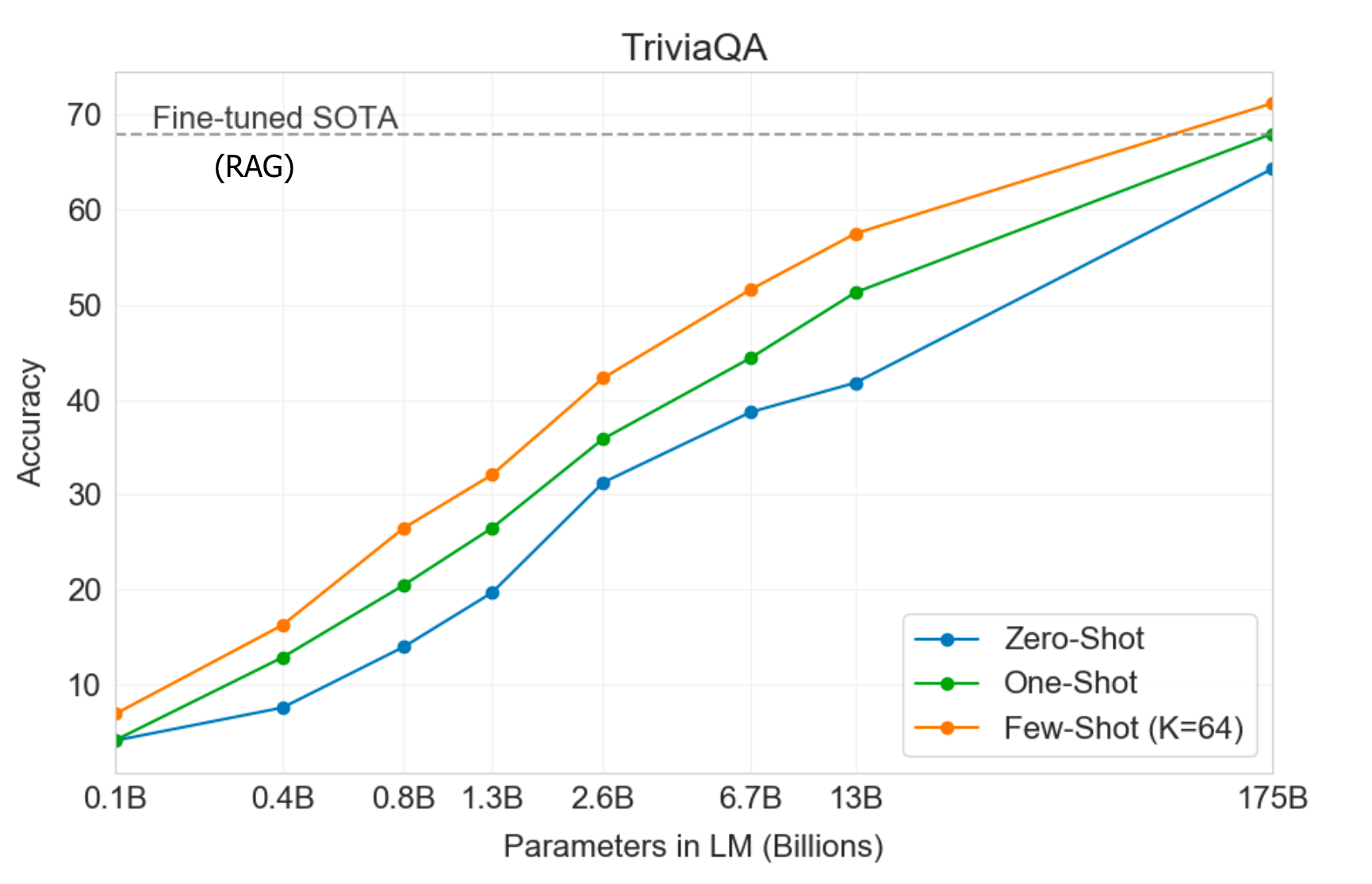
Interestingly, fine-tuning is not strictly necessary. GPT3 (Brown et al., 2020) has been evaluated on the closed book question answering task without any gradient updates or fine-tuning. During evaluation, the few-shot, one-shot and zero-shot settings here only refer to how many demonstrations are provided as context in the text input:
- “few-shot learning”: GPT3 is allowed to take as many demonstrations as what can fit into the model’s context window (typically 10 to 100).
- “one-shot learning”: only one demonstration is provided.
- “zero-shot learning”: no demonstrations are allowed and only an instruction in natural language is given to the model.
The performance grows with the model size. On the TriviaQA dataset, GPT3 evaluation with demonstrations can match or exceed the performance of SOTA baseline with fine-tuning.
Check out this cool example in OpenAI API playground viewer. The model is able to answer factal questions in short answer and not to make up things when the model does not know the answer. I added the last two questions and asked the model to respond with A:. The API is still in beta version, so you might need to apply to get on the wait list.
Q: Who is Batman?
A: Batman is a fictional comic book character.
##
Q: What is torsalplexity?
A: ?
##
Q: What is Devz9?
A: ?
##
Q: Who is George Lucas?
A: George Lucas is American film director and producer famous for creating Star Wars.
##
Q: What is the capital of California?
A: Sacramento.
##
Q: What orbits the Earth?
A: The Moon.
##
Q: Who is Fred Rickerson?
A: ?
##
Q: What is an atom?
A: An atom is a tiny particle that makes up everything.
##
Q: Who is Alvan Muntz?
A: ?
##
Q: What is Kozar-09?
A: ?
##
Q: How many moons does Mars have?
A: Two, Phobos and Deimos.
##
Q: What is COVID-19?
A: ?
##
Q: What is H1N1?
A: H1N1 is a strain of influenza.
Related Techniques
Fast Maximum Inner Product Search (MIPS)
MIPS (maximum inner product search) is a crucial component in many open-domain question answering models. In retriever + reader/generator framework, a large number of passages from the knowledge source are encoded and stored in a memory. A retrieval model is able to query the memory to identify the top relevant passages which have the maximum inner product with the question’s embedding.
We need fast MIPS because the number of precomputed passage representations can be gigantic. There are several ways to achieve fast MIPS at run time, such as asymmetric LSH, data-dependent hashing, and FAISS.
Language Model Pre-training
Two pre-training tasks are especially helpful for QA tasks, as we have discussed above.
-
Inverse Cloze Task (proposed by ORQA): The goal of Cloze Task is to predict masked-out text based on its context. The prediction of Inverse Cloze Task (ICT) is in the reverse direction, aiming to predict the context given a sentence. In the context of QA tasks, a random sentence can be treated as a pseudo-question, and its context can be treated as pseudo-evidence.
-
Salient Spans Masking (proposed by REALM): Salient span masking is a special case for MLM task in language model training. First, we find salient spans by using a tagger to identify named entities and a regular expression to identify dates. Then one of the detected salient spans is selected and masked. The task is to predict this masked salient span.
Summary
| Model | Retriever | Reader / Generator | Pre-training / Fine-tuning | End2end |
|---|---|---|---|---|
| DrQA | TF-IDF | Bi-directional LSTM | – | No |
| BERTserini | Aserini + BM25 | BERT without softmax layer | Fine-tune with SQuAD | No |
| Multi-passage BERT | ElasticSearch + BM25 | Multi-passage BERT + Passage ranker | No | |
| R^3 | Classic IR + Match-LSTM | Match-LSTM | Yes | |
| ORQA | Dot product of BERT embeddings | BERT-RC | Inverse cloze task | Yes |
| REALM | Dot product of BERT embeddings | BERT-RC | Salient span masking | Yes |
| DPR | Dot product of BERT embeddings | BERT-RC | supervised training with QA pairs | Yes |
| DenSPI | Classic + Neural IR | – | Yes | |
| T5 + SSM | – | T5 | SSM on CommonCrawl data + Fine-tuning on QA data | Yes |
| GPT3 | – | GPT3 | NSP on CommonCrawl data | Yes |
| RAG | DPR retriever | BART | Yes | |
| Fusion-in-Decoder | BM25 / DPR retriever | Tranformer | No |
Citation
Cited as:
Weng, Lilian. (Oct 2020). How to build an open-domain question answering system? Lil’Log. https://lilianweng.github.io/posts/2020-10-29-odqa/.
Or
@article{weng2020odqa,
  title   = "How to Build an Open-Domain Question Answering System?",
  author  = "Weng, Lilian",
  journal = "lilianweng.github.io",
  year    = "2020",
  month   = "Oct"
  url     = "https://lilianweng.github.io/posts/2020-10-29-odqa/"
}
Appendix: QA Datasets
- SQuAD 2.0: the Stanford QA dataset.
- RACE: a reading comprehension dataset collected from English Examinations that are created for middle school and high school students.
- TREC QA: the TREC QA collections.
- MS MARCO: a QA dataset featuring 100,000 real Bing questions and a human generated answer.
- CuratedTREC: based on the benchmarks from the TREC QA tasks that have been curated by Baudis & Sedivy (2015).
- Google Natural Questions: contains real user questions issued to Google search, and answers found from Wikipedia by annotators.
- WebQuestions: designed for knowledge-base QA with answers restricted to Freebase entities.
- WikiQA: Bing query logs were used as the source of questions. Each question is then linked to a Wikipedia page that potentially contains the answer.
- WikiMovies: contains movie-related questions from the OMDb and MovieLens databases and where the questions can be answered using Wikipedia pages.
- WikiReading: to predict textual values from the structured knowledge base Wikidata by reading the text of the corresponding Wikipedia articles.
- TriviaQA: a reading comprehension dataset containing 95K question-answer pairs authored by trivia enthusiasts and independently gathered multiple evidence documents per question.
- Jeopardy! Questions: contains 200,000+ Jeopardy! questions.
- DeepMind Q&A Dataset: question/answer pairs from CNN and Daily Mail articles.
- bAbi: a rich collection of datasets for text understanding by Facebook.
- FEVER: for fact extraction and verification.
- SearchQA: question-answer pairs were crawled from from J! Archive, and then augmented with text snippets from Google.
- Quasar-T: a collection of open-domain trivia questions and their answers obtained from various internet sources.
- Quiz bowl: contains data from a trivia competition called quiz bowl.
- AmbigNQ: ambiguous questions selected from NQ-OPEN dataset.
- QA-Overlap: a collections of overlapped answers/questions between train and test set for Natural Questions, TriviaQA, and WebQuestions.
References
[1] Danqi Chen & Scott Yih. “ACL2020 Tutorial: Open-Domain Question Answering” July 2020.
[2] Danqi Chen, et al. “Reading Wikipedia to Answer Open-Domain Questions” ACL 2017. | code
[3] Shuohang Wang, et al. “R^3: Reinforced Ranker-Reader for Open-Domain Question Answering” AAAI 2018.
[4] Jimmy Lin. “The neural hype and comparisons against weak baselines.” ACM SIGIR Forum. Vol. 52. No. 2. 2019.
[5] Wei Yang, et al. “End-to-End Open-Domain Question Answering with BERTserini” NAACL 2019.
[6] Christopher Clark & Matt Gardner. “Simple and Effective Multi-Paragraph Reading Comprehension.” arXiv:1710.10723 (2017).
[7] Rodrigo Nogueira & Kyunghyun Cho. “Passage Re-ranking with BERT.” arXiv preprint arXiv:1901.04085 (2019). | code
[8] Zhiguo Wang, et al. “Multi-passage BERT: A globally normalized BERT model for open-domain question answering.” EMNLP 2019.
[9] Minjoon Seo et al. “Real-time open-domain question answering with dense-sparse phrase index.” ACL 2019.
[10] Kenton Lee, et al. “Latent Retrieval for Weakly Supervised Open Domain Question Answering” ACL 2019.
[11] Kelvin Guu, et al. “REALM: Retrieval-Augmented Language Model Pre-Training” arXiv:2002.08909 (2020).
[12] Vladimir Karpukhin et al. “Dense passage retrieval for open-domain question answering.”. EMNLP 2020. | code
[13] Patrick Lewis et al. “Retrieval-Augmented Generation for Knowledge-Intensive NLP Tasks” arXiv:2005.11401 (2020).
[14] Adam Roberts, et al. “How Much Knowledge Can You Pack Into the Parameters of a Language Model?” EMNLP 2020.
[15] Tom Brown, et al. “Language models are few-shot learners.” arXiv:2005.14165 (2020).
[16] Fabio Petroni, et al. “How Context Affects Language Models’ Factual Predictions” AKBC 2020.
[17] Gautier Izacard & Edouard Grave. “Leveraging passage retrieval with generative models for open domain question answering.” arXiv:2007.01282 (2020).
[18] “Dive into deep learning: Beam search”
[19] Patrick Lewis, et al. “Question and Answer Test-Train Overlap in Open-Domain Question Answering Datasets” arXiv:2008.02637 (2020). | data
[20] Hervé Jegou, et al. “Faiss: A library for efficient similarity search” Mar 2017.
[21] Vidhisha Balachandran, et al. “Simple and Efficient ways to Improve REALM.” arXiv:2104.08710 (2021).