Human vocabulary comes in free text. In order to make a machine learning model understand and process the natural language, we need to transform the free-text words into numeric values. One of the simplest transformation approaches is to do a one-hot encoding in which each distinct word stands for one dimension of the resulting vector and a binary value indicates whether the word presents (1) or not (0).
However, one-hot encoding is impractical computationally when dealing with the entire vocabulary, as the representation demands hundreds of thousands of dimensions. Word embedding represents words and phrases in vectors of (non-binary) numeric values with much lower and thus denser dimensions. An intuitive assumption for good word embedding is that they can approximate the similarity between words (i.e., “cat” and “kitten” are similar words, and thus they are expected to be close in the reduced vector space) or disclose hidden semantic relationships (i.e., the relationship between “cat” and “kitten” is an analogy to the one between “dog” and “puppy”). Contextual information is super useful for learning word meaning and relationship, as similar words may appear in the similar context often.
There are two main approaches for learning word embedding, both relying on the contextual knowledge.
- Count-based: The first one is unsupervised, based on matrix factorization of a global word co-occurrence matrix. Raw co-occurrence counts do not work well, so we want to do smart things on top.
- Context-based: The second approach is supervised. Given a local context, we want to design a model to predict the target words and in the meantime, this model learns the efficient word embedding representation.
Count-Based Vector Space Model
Count-based vector space models heavily rely on the word frequency and co-occurrence matrix with the assumption that words in the same contexts share similar or related semantic meanings. The models map count-based statistics like co-occurrences between neighboring words down to a small and dense word vectors. PCA, topic models, and neural probabilistic language models are all good examples of this category.
Different from the count-based approaches, context-based methods build predictive models that directly target at predicting a word given its neighbors. The dense word vectors are part of the model parameters. The best vector representation of each word is learned during the model training process.
Context-Based: Skip-Gram Model
Suppose that you have a sliding window of a fixed size moving along a sentence: the word in the middle is the “target” and those on its left and right within the sliding window are the context words. The skip-gram model (Mikolov et al., 2013) is trained to predict the probabilities of a word being a context word for the given target.
The following example demonstrates multiple pairs of target and context words as training samples, generated by a 5-word window sliding along the sentence.
“The man who passes the sentence should swing the sword.” – Ned Stark
| Sliding window (size = 5) | Target word | Context |
|---|---|---|
| [The man who] | the | man, who |
| [The man who passes] | man | the, who, passes |
| [The man who passes the] | who | the, man, passes, the |
| [man who passes the sentence] | passes | man, who, the, sentence |
| … | … | … |
| [sentence should swing the sword] | swing | sentence, should, the, sword |
| [should swing the sword] | the | should, swing, sword |
| [swing the sword] | sword | swing, the |
| {:.info} |
Each context-target pair is treated as a new observation in the data. For example, the target word “swing” in the above case produces four training samples: (“swing”, “sentence”), (“swing”, “should”), (“swing”, “the”), and (“swing”, “sword”).
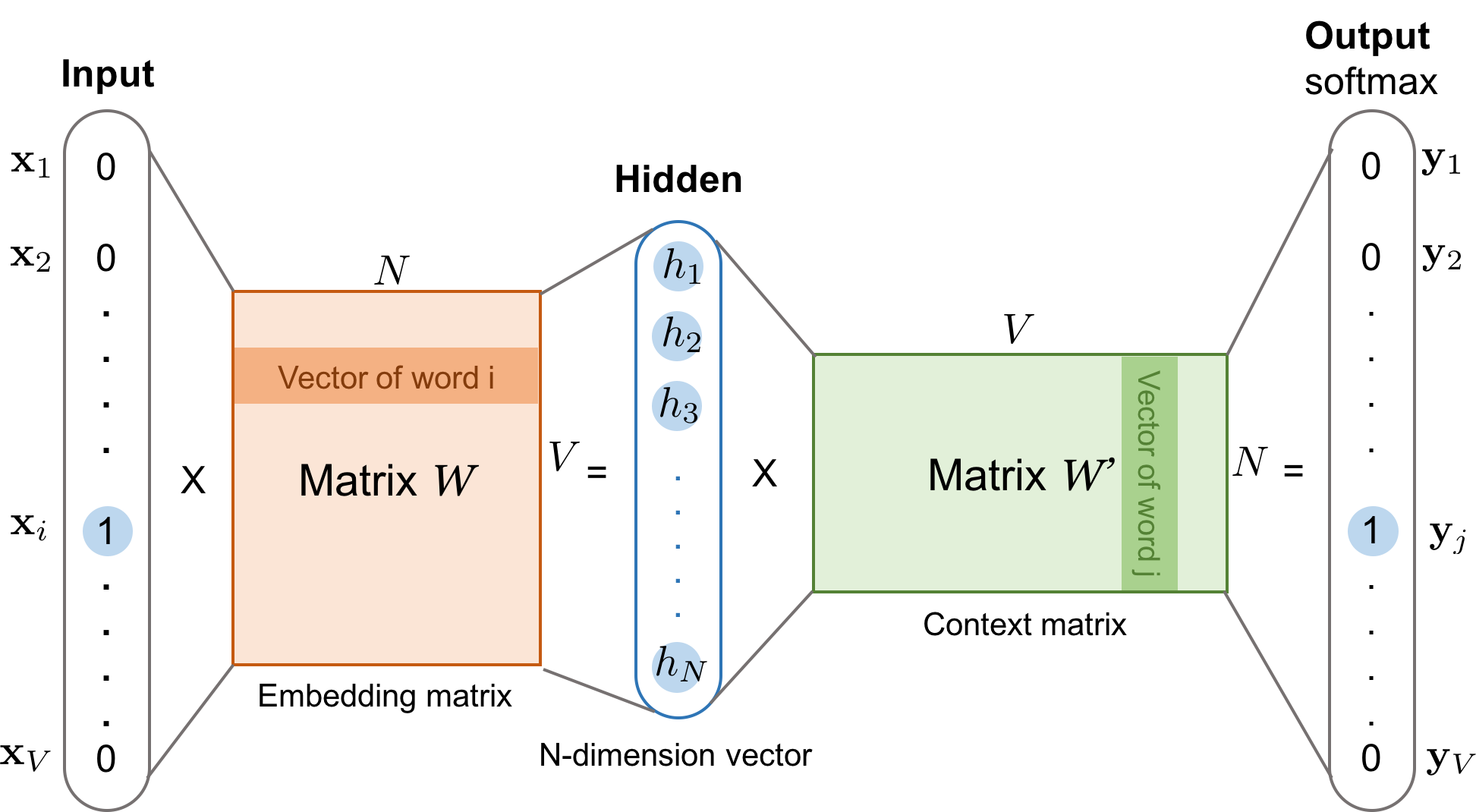
Given the vocabulary size $V$, we are about to learn word embedding vectors of size $N$. The model learns to predict one context word (output) using one target word (input) at a time.
According to Fig. 1,
- Both input word $w_i$ and the output word $w_j$ are one-hot encoded into binary vectors $\mathbf{x}$ and $\mathbf{y}$ of size $V$.
- First, the multiplication of the binary vector $\mathbf{x}$ and the word embedding matrix $W$ of size $V \times N$ gives us the embedding vector of the input word $w_i$: the i-th row of the matrix $W$.
- This newly discovered embedding vector of dimension $N$ forms the hidden layer.
- The multiplication of the hidden layer and the word context matrix $W’$ of size $N \times V$ produces the output one-hot encoded vector $\mathbf{y}$.
- The output context matrix $W’$ encodes the meanings of words as context, different from the embedding matrix $W$. NOTE: Despite the name, $W’$ is independent of $W$, not a transpose or inverse or whatsoever.
Context-Based: Continuous Bag-of-Words (CBOW)
The Continuous Bag-of-Words (CBOW) is another similar model for learning word vectors. It predicts the target word (i.e. “swing”) from source context words (i.e., “sentence should the sword”).
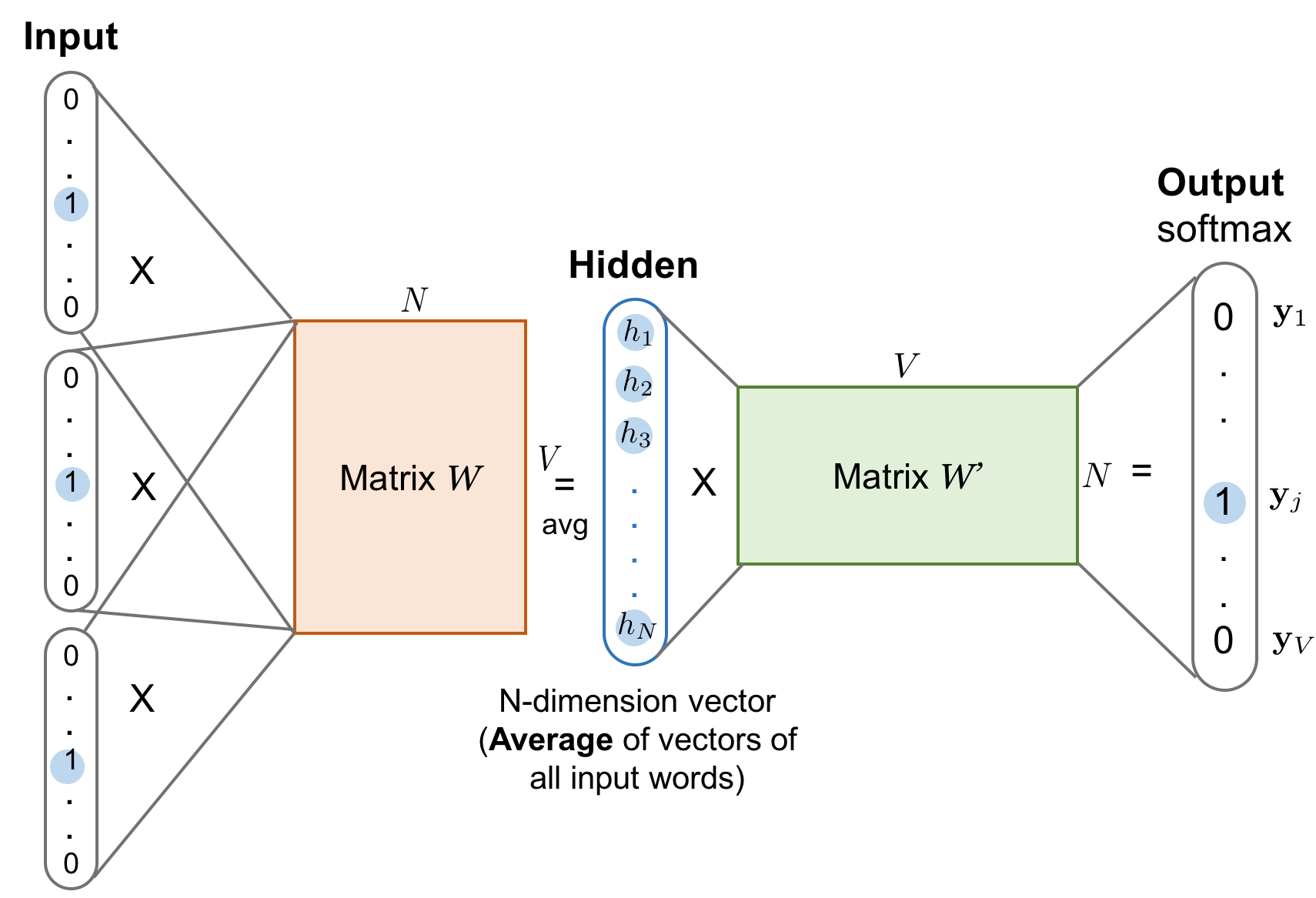
Because there are multiple contextual words, we average their corresponding word vectors, constructed by the multiplication of the input vector and the matrix $W$. Because the averaging stage smoothes over a lot of the distributional information, some people believe the CBOW model is better for small dataset.
Loss Functions
Both the skip-gram model and the CBOW model should be trained to minimize a well-designed loss/objective function. There are several loss functions we can incorporate to train these language models. In the following discussion, we will use the skip-gram model as an example to describe how the loss is computed.
Full Softmax
The skip-gram model defines the embedding vector of every word by the matrix $W$ and the context vector by the output matrix $W’$. Given an input word $w_I$, let us label the corresponding row of $W$ as vector $v_{w_I}$ (embedding vector) and its corresponding column of $W’$ as $v’_{w_I}$ (context vector). The final output layer applies softmax to compute the probability of predicting the output word $w_O$ given $w_I$, and therefore:
This is accurate as presented in However, when $V$ is extremely large, calculating the denominator by going through all the words for every single sample is computationally impractical. The demand for more efficient conditional probability estimation leads to the new methods like hierarchical softmax.
Hierarchical Softmax
Morin and Bengio (2005) proposed hierarchical softmax to make the sum calculation faster with the help of a binary tree structure. The hierarchical softmax encodes the language model’s output softmax layer into a tree hierarchy, where each leaf is one word and each internal node stands for relative probabilities of the children nodes.
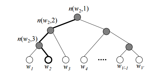
Each word $w_i$ has a unique path from the root down to its corresponding leaf. The probability of picking this word is equivalent to the probability of taking this path from the root down through the tree branches. Since we know the embedding vector $v_n$ of the internal node $n$, the probability of getting the word can be computed by the product of taking left or right turn at every internal node stop.
According to Fig. 3, the probability of one node is ($\sigma$ is the sigmoid function):
The final probability of getting a context word $w_O$ given an input word $w_I$ is:
where $L(w_O)$ is the depth of the path leading to the word $w_O$ and $\mathbb{I}_{\text{turn}}$ is a specially indicator function which returns 1 if $n(w_O, k+1)$ is the left child of $n(w_O, k)$ otherwise -1. The internal nodes’ embeddings are learned during the model training. The tree structure helps greatly reduce the complexity of the denominator estimation from O(V) (vocabulary size) to O(log V) (the depth of the tree) at the training time. However, at the prediction time, we still to compute the probability of every word and pick the best, as we don’t know which leaf to reach for in advance.
A good tree structure is crucial to the model performance. Several handy principles are: group words by frequency like what is implemented by Huffman tree for simple speedup; group similar words into same or close branches (i.e. use predefined word clusters, WordNet).
Cross Entropy
Another approach completely steers away from the softmax framework. Instead, the loss function measures the cross entropy between the predicted probabilities $p$ and the true binary labels $\mathbf{y}$.
First, let’s recall that the cross entropy between two distributions $p$ and $q$ is measured as $ H(p, q) = -\sum_x p(x) \log q(x) $. In our case, the true label $y_i$ is 1 only when $w_i$ is the output word; $y_j$ is 0 otherwise. The loss function $\mathcal{L}_\theta$ of the model with parameter config $\theta$ aims to minimize the cross entropy between the prediction and the ground truth, as lower cross entropy indicates high similarity between two distributions.
Recall that,
Therefore,
To start training the model using back-propagation with SGD, we need to compute the gradient of the loss function. For simplicity, let’s label $z_{IO} = {v’_{w_O}}^{\top}{v_{w_I}}$.
where $Q(\tilde{w})$ is the distribution of noise samples.
According to the formula above, the correct output word has a positive reinforcement according to the first term (the larger $\nabla_\theta z_{IO}$ the better loss we have), while other words have a negative impact as captured by the second term.
How to estimate $\mathbb{E}_{w_i \sim Q(\tilde{w})} \nabla_\theta {v’_{w_i}}^{\top}{v_{w_I}}$ with a sample set of noise words rather than scanning through the entire vocabulary is the key of using cross-entropy-based sampling approach.
Noise Contrastive Estimation (NCE)
The Noise Contrastive Estimation (NCE) metric intends to differentiate the target word from noise samples using a logistic regression classifier (Gutmann and Hyvärinen, 2010).
Given an input word $w_I$, the correct output word is known as $w$. In the meantime, we sample $N$ other words from the noise sample distribution $Q$, denoted as $\tilde{w}_1, \tilde{w}_2, \dots, \tilde{w}_N \sim Q$. Let’s label the decision of the binary classifier as $d$ and $d$$ can only take a binary value.
When $N$ is big enough, according to the Law of large numbers,
To compute the probability $p(d=1 \vert w, w_I)$, we can start with the joint probability $p(d, w \vert w_I)$. Among $w, \tilde{w}_1, \tilde{w}_2, \dots, \tilde{w}_N$, we have 1 out of (N+1) chance to pick the true word $w$, which is sampled from the conditional probability $p(w \vert w_I)$; meanwhile, we have N out of (N+1) chances to pick a noise word, each sampled from $q(\tilde{w}) \sim Q$. Thus,
Then we can figure out $p(d=1 \vert w, w_I)$ and $p(d=0 \vert w, w_I)$:
Finally the loss function of NCE’s binary classifier becomes:
However, $p(w \vert w_I)$ still involves summing up the entire vocabulary in the denominator. Let’s label the denominator as a partition function of the input word, $Z(w_I)$. A common assumption is $Z(w) \approx 1$ given that we expect the softmax output layer to be normalized (Minh and Teh, 2012). Then the loss function is simplified to:
The noise distribution $Q$ is a tunable parameter and we would like to design it in a way so that:
- intuitively it should be very similar to the real data distribution; and
- it should be easy to sample from.
For example, the sampling implementation (log_uniform_candidate_sampler) of NCE loss in tensorflow assumes that such noise samples follow a log-uniform distribution, also known as Zipfian’s law. The probability of a given word in logarithm is expected to be reversely proportional to its rank, while high-frequency words are assigned with lower ranks. In this case, $q(\tilde{w}) = \frac{1}{ \log V}(\log (r_{\tilde{w}} + 1) - \log r_{\tilde{w}})$, where $r_{\tilde{w}} \in [1, V]$ is the rank of a word by frequency in descending order.
Negative Sampling (NEG)
The Negative Sampling (NEG) proposed by Mikolov et al. (2013) is a simplified variation of NCE loss. It is especially famous for training Google’s word2vec project. Different from NCE Loss which attempts to approximately maximize the log probability of the softmax output, negative sampling did further simplification because it focuses on learning high-quality word embedding rather than modeling the word distribution in natural language.
NEG approximates the binary classifier’s output with sigmoid functions as follows:
The final NCE loss function looks like:
Other Tips for Learning Word Embedding
Mikolov et al. (2013) suggested several helpful practices that could result in good word embedding learning outcomes.
-
Soft sliding window. When pairing the words within the sliding window, we could assign less weight to more distant words. One heuristic is — given a maximum window size parameter defined, $s_{\text{max}}$, the actual window size is randomly sampled between 1 and $s_{\text{max}}$ for every training sample. Thus, each context word has the probability of 1/(its distance to the target word) being observed, while the adjacent words are always observed.
-
Subsampling frequent words. Extremely frequent words might be too general to differentiate the context (i.e. think about stopwords). While on the other hand, rare words are more likely to carry distinct information. To balance the frequent and rare words, Mikolov et al. proposed to discard words $w$ with probability $1-\sqrt{t/f(w)}$ during sampling. Here $f(w)$ is the word frequency and $t$ is an adjustable threshold.
-
Learning phrases first. A phrase often stands as a conceptual unit, rather than a simple composition of individual words. For example, we cannot really tell “New York” is a city name even we know the meanings of “new” and “york”. Learning such phrases first and treating them as word units before training the word embedding model improves the outcome quality. A simple data-driven approach is based on unigram and bigram counts: $s_{\text{phrase}} = \frac{C(w_i w_j) - \delta}{ C(w_i)C(w_j)}$, where $C(.)$ is simple count of an unigram $w_i$ or bigram $w_i w_j$ and $\delta$ is a discounting threshold to prevent super infrequent words and phrases. Higher scores indicate higher chances of being phrases. To form phrases longer than two words, we can scan the vocabulary multiple times with decreasing score cutoff values.
GloVe: Global Vectors
The Global Vector (GloVe) model proposed by Pennington et al. (2014) aims to combine the count-based matrix factorization and the context-based skip-gram model together.
We all know the counts and co-occurrences can reveal the meanings of words. To distinguish from $p(w_O \vert w_I)$ in the context of a word embedding word, we would like to define the co-ocurrence probability as:
$C(w_i, w_k)$ counts the co-occurrence between words $w_i$ and $w_k$.
Say, we have two words, $w_i$=“ice” and $w_j$=“steam”. The third word $\tilde{w}_k$=“solid” is related to “ice” but not “steam”, and thus we expect $p_{\text{co}}(\tilde{w}_k \vert w_i)$ to be much larger than $p_{\text{co}}(\tilde{w}_k \vert w_j)$ and therefore $\frac{p_{\text{co}}(\tilde{w}_k \vert w_i)}{p_{\text{co}}(\tilde{w}_k \vert w_j)}$ to be very large. If the third word $\tilde{w}_k$ = “water” is related to both or $\tilde{w}_k$ = “fashion” is unrelated to either of them, $\frac{p_{\text{co}}(\tilde{w}_k \vert w_i)}{p_{\text{co}}(\tilde{w}_k \vert w_j)}$ is expected to be close to one.
The intuition here is that the word meanings are captured by the ratios of co-occurrence probabilities rather than the probabilities themselves. The global vector models the relationship between two words regarding to the third context word as:
Further, since the goal is to learn meaningful word vectors, $F$ is designed to be a function of the linear difference between two words $w_i - w_j$:
With the consideration of $F$ being symmetric between target words and context words, the final solution is to model $F$ as an exponential function. Please read the original paper (Pennington et al., 2014) for more details of the equations.
Finally,
Since the second term $-\log C(w_i)$ is independent of $k$, we can add bias term $b_i$ for $w_i$ to capture $-\log C(w_i)$. To keep the symmetric form, we also add in a bias $\tilde{b}_k$ for $\tilde{w}_k$.
The loss function for the GloVe model is designed to preserve the above formula by minimizing the sum of the squared errors:
The weighting schema $f(c)$ is a function of the co-occurrence of $w_i$ and $w_j$ and it is an adjustable model configuration. It should be close to zero as $c \to 0$; should be non-decreasing as higher co-occurrence should have more impact; should saturate when $c$ become extremely large. The paper proposed the following weighting function.
Examples: word2vec on “Game of Thrones”
After reviewing all the theoretical knowledge above, let’s try a little experiment in word embedding extracted from “the Games of Thrones corpus”. The process is super straightforward using gensim.
Step 1: Extract words
import sys
from nltk.corpus import stopwords
from nltk.tokenize import sent_tokenize

STOP_WORDS = set(stopwords.words('english'))

def get_words(txt):
    return filter(
        lambda x: x not in STOP_WORDS,
        re.findall(r'\b(\w+)\b', txt)
    )

def parse_sentence_words(input_file_names):
   """Returns a list of a list of words. Each sublist is a sentence."""
    sentence_words = []
    for file_name in input_file_names:
        for line in open(file_name):
            line = line.strip().lower()
            line = line.decode('unicode_escape').encode('ascii','ignore')
            sent_words = map(get_words, sent_tokenize(line))
            sent_words = filter(lambda sw: len(sw) > 1, sent_words)
            if len(sent_words) > 1:
                sentence_words += sent_words
    return sentence_words

# You would see five .txt files after unzip 'a_song_of_ice_and_fire.zip'
input_file_names = ["001ssb.txt", "002ssb.txt", "003ssb.txt",
                    "004ssb.txt", "005ssb.txt"]
GOT_SENTENCE_WORDS= parse_sentence_words(input_file_names)
Step 2: Feed a word2vec model
from gensim.models import Word2Vec

# size: the dimensionality of the embedding vectors.
# window: the maximum distance between the current and predicted word within a sentence.
model = Word2Vec(GOT_SENTENCE_WORDS, size=128, window=3, min_count=5, workers=4)
model.wv.save_word2vec_format("got_word2vec.txt", binary=False)
Step 3: Check the results
In the GoT word embedding space, the top similar words to “king” and “queen” are:
model.most_similar('king', topn=10)(word, similarity with ‘king’) |
model.most_similar('queen', topn=10)(word, similarity with ‘queen’) |
|---|---|
| (‘kings’, 0.897245) | (‘cersei’, 0.942618) |
| (‘baratheon’, 0.809675) | (‘joffrey’, 0.933756) |
| (‘son’, 0.763614) | (‘margaery’, 0.931099) |
| (‘robert’, 0.708522) | (‘sister’, 0.928902) |
| (’lords’, 0.698684) | (‘prince’, 0.927364) |
| (‘joffrey’, 0.696455) | (‘uncle’, 0.922507) |
| (‘prince’, 0.695699) | (‘varys’, 0.918421) |
| (‘brother’, 0.685239) | (’ned’, 0.917492) |
| (‘aerys’, 0.684527) | (‘melisandre’, 0.915403) |
| (‘stannis’, 0.682932) | (‘robb’, 0.915272) |
Cited as:
@article{weng2017wordembedding,
  title   = "Learning word embedding",
  author  = "Weng, Lilian",
  journal = "lilianweng.github.io",
  year    = "2017",
  url     = "https://lilianweng.github.io/posts/2017-10-15-word-embedding/"
}
References
[1] Tensorflow Tutorial Vector Representations of Words.
[2] “Word2Vec Tutorial - The Skip-Gram Model” by Chris McCormick.
[3] “On word embeddings - Part 2: Approximating the Softmax” by Sebastian Ruder.
[4] Xin Rong. word2vec Parameter Learning Explained
[5] Mikolov, Tomas, Kai Chen, Greg Corrado, and Jeffrey Dean. “Efficient estimation of word representations in vector space.” arXiv preprint arXiv:1301.3781 (2013).
[6] Frederic Morin and Yoshua Bengio. “Hierarchical Probabilistic Neural Network Language Model.” Aistats. Vol. 5. 2005.
[7] Michael Gutmann and Aapo Hyvärinen. “Noise-contrastive estimation: A new estimation principle for unnormalized statistical models.” Proc. Intl. Conf. on Artificial Intelligence and Statistics. 2010.
[8] Tomas Mikolov, Ilya Sutskever, Kai Chen, Greg Corrado, and Jeffrey Dean. “Distributed representations of words and phrases and their compositionality.” Advances in neural information processing systems. 2013.
[9] Tomas Mikolov, Kai Chen, Greg Corrado, and Jeffrey Dean. “Efficient estimation of word representations in vector space.” arXiv preprint arXiv:1301.3781 (2013).
[10] Marco Baroni, Georgiana Dinu, and Germán Kruszewski. “Don’t count, predict! A systematic comparison of context-counting vs. context-predicting semantic vectors.” ACL (1). 2014.
[11] Jeffrey Pennington, Richard Socher, and Christopher Manning. “Glove: Global vectors for word representation.” Proc. Conf. on empirical methods in natural language processing (EMNLP). 2014.