Professor Naftali Tishby passed away in 2021. Hope the post can introduce his cool idea of information bottleneck to more people.
Recently I watched the talk “Information Theory in Deep Learning” by Prof Naftali Tishby and found it very interesting. He presented how to apply the information theory to study the growth and transformation of deep neural networks during training. Using the Information Bottleneck (IB) method, he proposed a new learning bound for deep neural networks (DNN), as the traditional learning theory fails due to the exponentially large number of parameters. Another keen observation is that DNN training involves two distinct phases: First, the network is trained to fully represent the input data and minimize the generalization error; then, it learns to forget the irrelevant details by compressing the representation of the input.
Most of the materials in this post are from Prof Tishby’s talk and related papers.
Basic Concepts
A Markov process is a “memoryless” (also called “Markov Property”) stochastic process. A Markov chain is a type of Markov process containing multiple discrete states. That is being said, the conditional probability of future states of the process is only determined by the current state and does not depend on the past states.
Kullback–Leibler (KL) Divergence
KL divergence measures how one probability distribution $p$ diverges from a second expected probability distribution $q$. It is asymmetric.
$D_{KL}$ achieves the minimum zero when $p(x)$ == $q(x)$ everywhere.
Mutual information measures the mutual dependence between two variables. It quantifies the “amount of information” obtained about one random variable through the other random variable. Mutual information is symmetric.
Data Processing Inequality (DPI)
For any markov chain: $X \to Y \to Z$, we would have $I(X; Y) \geq I(X; Z)$.
A deep neural network can be viewed as a Markov chain, and thus when we are moving down the layers of a DNN, the mutual information between the layer and the input can only decrease.
For two invertible functions $\phi$, $\psi$, the mutual information still holds: $I(X; Y) = I(\phi(X); \psi(Y))$.
For example, if we shuffle the weights in one layer of DNN, it would not affect the mutual information between this layer and another.
Deep Neural Networks as Markov Chains
The training data contains sampled observations from the joint distribution of $X$ and $Y$. The input variable $X$ and weights of hidden layers are all high-dimensional random variable. The ground truth target $Y$ and the predicted value $\hat{Y}$ are random variables of smaller dimensions in the classification settings.
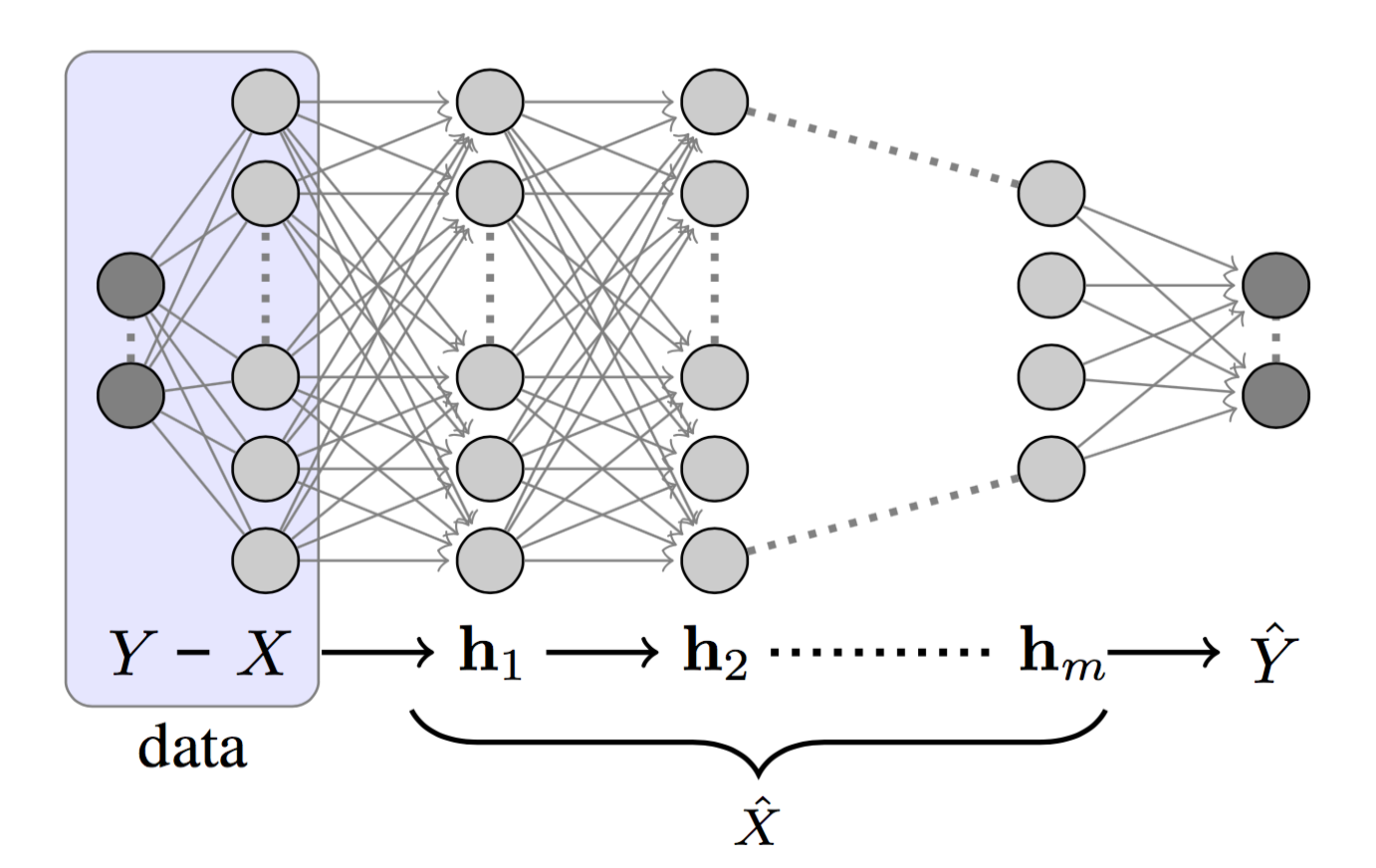
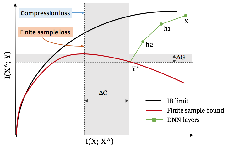
If we label the hidden layers of a DNN as $h_1, h_2, \dots, h_m$ as in Fig. 1, we can view each layer as one state of a Markov Chain: $ h_i \to h_{i+1}$. According to DPI, we would have:
A DNN is designed to learn how to describe $X$ to predict $Y$ and eventually, to compress $X$ to only hold the information related to $Y$. Tishby describes this processing as “successive refinement of relevant information”.
Information Plane Theorem
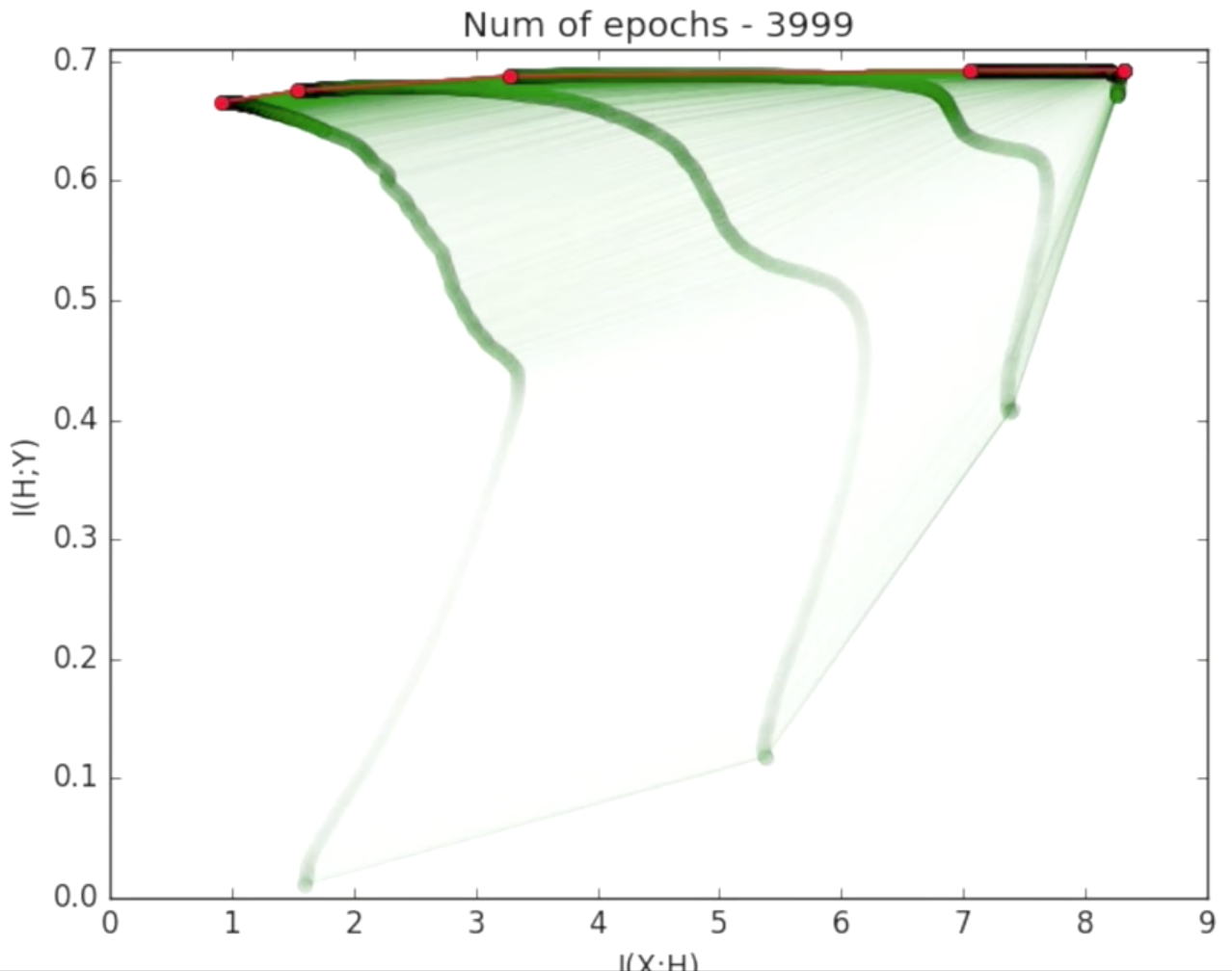
A DNN has successive internal representations of $X$, a set of hidden layers $\{T_i\}$. The information plane theorem characterizes each layer by its encoder and decoder information. The encoder is a representation of the input data $X$, while the decoder translates the information in the current layer to the target ouput $Y$.
Precisely, in an information plane plot:
- X-axis: The sample complexity of $T_i$ is determined by the encoder mutual information $I(X; T_i)$. Sample complexity refers to how many samples you need to achieve certain accuracy and generalization.
- Y-axis: The accuracy (generalization error) is determined by the decoder mutual information $I(T_i; Y)$.
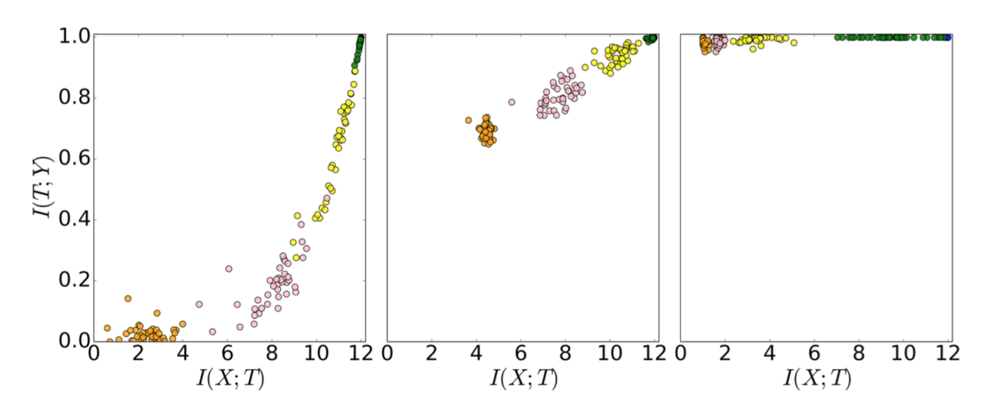
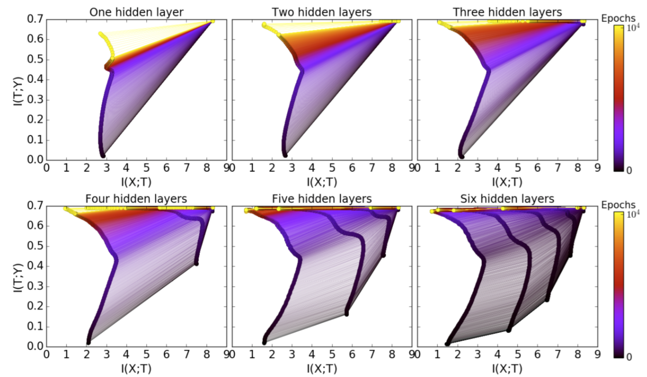
Each dot in marks the encoder/ decoder mutual information of one hidden layer of one network simulation (no regularization is applied; no weights decay, no dropout, etc.). They move up as expected because the knowledge about the true labels is increasing (accuracy increases). At the early stage, the hidden layers learn a lot about the input $X$, but later they start to compress to forget some information about the input. Tishby believes that “the most important part of learning is actually forgetting”. Check out this nice video that demonstrates how the mutual information measures of layers are changing in epoch time.
Two Optimization Phases
Tracking the normalized mean and standard deviation of each layer’s weights in time also reveals two optimization phases of the training process.
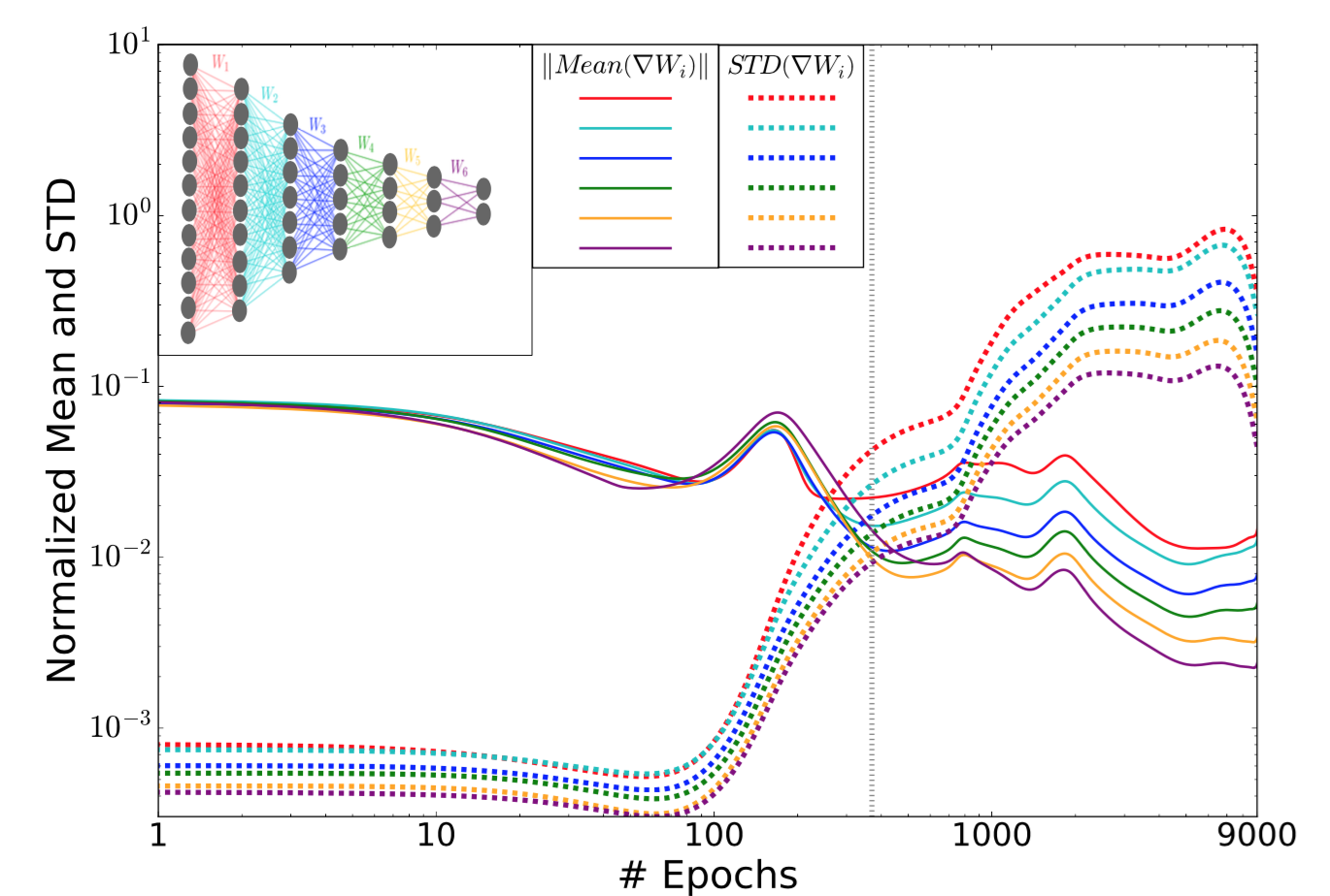
Among early epochs, the mean values are three magnitudes larger than the standard deviations. After a sufficient number of epochs, the error saturates and the standard deviations become much noisier afterward. The further a layer is away from the output, the noisier it gets, because the noises can get amplified and accumulated through the back-prop process (not due to the width of the layer).
Learning Theory
“Old” Generalization Bounds
The generalization bounds defined by the classic learning theory is:
- $\epsilon$: The difference between the training error and the generalization error. The generalization error measures how accurate the prediction of an algorithm is for previously unseen data.
- $H_\epsilon$: $\epsilon$-cover of the hypothesis class. Typically we assume the size $\vert H_\epsilon \vert \sim (1/\epsilon)^d$.
- $\delta$: Confidence.
- $m$: The number of training samples.
- $d$: The VC dimension of the hypothesis.
This definition states that the difference between the training error and the generalization error is bounded by a function of the hypothesis space size and the dataset size. The bigger the hypothesis space gets, the bigger the generalization error becomes. I recommend this tutorial on ML theory, part1 and part2, if you are interested in reading more on generalization bounds.
However, it does not work for deep learning. The larger a network is, the more parameters it needs to learn. With this generalization bounds, larger networks (larger $d$) would have worse bounds. This is contrary to the intuition that larger networks are able to achieve better performance with higher expressivity.
“New” Input compression bound
To solve this counterintuitive observation, Tishby et al. proposed a new input compression bound for DNN.
First let us have $T_\epsilon$ as an $\epsilon$-partition of the input variable $X$. This partition compresses the input with respect to the homogeneity to the labels into small cells. The cells in total can cover the whole input space. If the prediction outputs binary values, we can replace the cardinality of the hypothesis, $\vert H_\epsilon \vert$, with $2^{\vert T_\epsilon \vert}$.
When $X$ is large, the size of $X$ is approximately $2^{H(X)}$. Each cell in the $\epsilon$-partition is of size $2^{H(X \vert T_\epsilon)}$. Therefore we have $\vert T_\epsilon \vert \sim \frac{2^{H(X)}}{2^{H(X \vert T_\epsilon)}} = 2^{I(T_\epsilon; X)}$. Then the input compression bound becomes:
Network Size and Training Data Size
The Benefit of More Hidden Layers
Having more layers give us computational benefits and speed up the training process for good generalization.
Compression through stochastic relaxation: According to the diffusion equation, the relaxation time of layer $k$ is proportional to the exponential of this layer’s compression amount $\Delta S_k$: $\Delta t_k \sim \exp(\Delta S_k)$. We can compute the layer compression as $\Delta S_k = I(X; T_k) - I(X; T_{k-1})$. Because $\exp(\sum_k \Delta S_k) \geq \sum_k \exp(\Delta S_k)$, we would expect an exponential decrease in training epochs with more hidden layers (larger $k$).
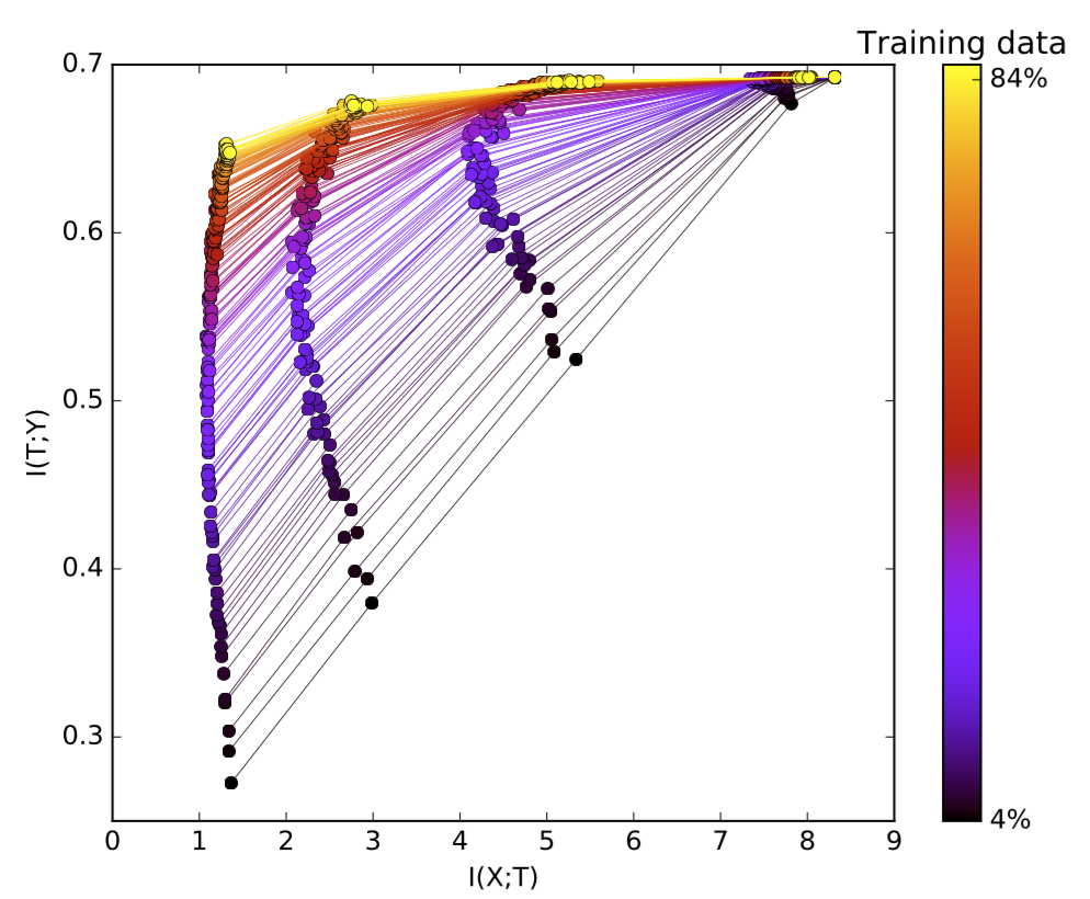
The Benefit of More Training Samples
Fitting more training data requires more information captured by the hidden layers. With increased training data size, the decoder mutual information (recall that this is directly related to the generalization error), $I(T; Y)$, is pushed up and gets closer to the theoretical information bottleneck bound. Tishby emphasized that It is the mutual information, not the layer size or the VC dimension, that determines generalization, different from standard theories.
Cited as:
@article{weng2017infotheory,
  title   = "Anatomize Deep Learning with Information Theory",
  author  = "Weng, Lilian",
  journal = "lilianweng.github.io",
  year    = "2017",
  url     = "https://lilianweng.github.io/posts/2017-09-28-information-bottleneck/"
}
References
[1] Naftali Tishby. Information Theory of Deep Learning
[2] Machine Learning Theory - Part 1: Introduction
[3] Machine Learning Theory - Part 2: Generalization Bounds
[4] New Theory Cracks Open the Black Box of Deep Learning by Quanta Magazine.
[5] Naftali Tishby and Noga Zaslavsky. “Deep learning and the information bottleneck principle.” IEEE Information Theory Workshop (ITW), 2015.
[6] Ravid Shwartz-Ziv and Naftali Tishby. “Opening the Black Box of Deep Neural Networks via Information.” arXiv preprint arXiv:1703.00810, 2017.