In Robotics, one of the hardest problems is how to make your model transfer to the real world. Due to the sample inefficiency of deep RL algorithms and the cost of data collection on real robots, we often need to train models in a simulator which theoretically provides an infinite amount of data. However, the reality gap between the simulator and the physical world often leads to failure when working with physical robots. The gap is triggered by an inconsistency between physical parameters (i.e. friction, kp, damping, mass, density) and, more fatally, the incorrect physical modeling (i.e. collision between soft surfaces).

To close the sim2real gap, we need to improve the simulator and make it closer to reality. A couple of approaches:

System identification
- System identification is to build a mathematical model for a physical system; in the context of RL, the mathematical model is the simulator. To make the simulator more realistic, careful calibration is necessary.
- Unfortunately, calibration is expensive. Furthermore, many physical parameters of the same machine might vary significantly due to temperature, humidity, positioning or its wear-and-tear in time.
Domain adaptation
- Domain adaptation (DA) refers to a set of transfer learning techniques developed to update the data distribution in sim to match the real one through a mapping or regularization enforced by the task model.
- Many DA models, especially for image classification or end-to-end image-based RL task, are built on adversarial loss or GAN.
Domain randomization
- With domain randomization (DR), we are able to create a variety of simulated environments with randomized properties and train a model that works across all of them.
- Likely this model can adapt to the real-world environment, as the real system is expected to be one sample in that rich distribution of training variations.

Both DA and DR are unsupervised. Compared to DA which requires a decent amount of real data samples to capture the distribution, DR may need only a little or no real data. DR is the focus of this post.

Fig. 1. Conceptual illustrations of three approaches for sim2real transfer.

What is Domain Randomization?

To make the definition more general, let us call the environment that we have full access to (i.e. simulator) source domain and the environment that we would like to transfer the model to target domain (i.e. physical world). Training happens in the source domain. We can control a set of $N$ randomization parameters in the source domain $e_\xi$ with a configuration $\xi$, sampled from a randomization space, $\xi \in \Xi \subset \mathbb{R}^N$.

During policy training, episodes are collected from source domain with randomization applied. Thus the policy is exposed to a variety of environments and learns to generalize. The policy parameter $\theta$ is trained to maximize the expected reward $R(.)$ average across a distribution of configurations:

$$ \theta^* = \arg\max_\theta \mathbb{E}_{\xi \sim \Xi} [\mathbb{E}_{\pi_\theta, \tau \sim e_\xi} [R(\tau)]] $$

where $\tau_\xi$ is a trajectory collected in source domain randomized with $\xi$. In a way, “discrepancies between the source and target domains are modeled as variability in the source domain.” (quote from Peng et al. 2018).

Uniform Domain Randomization

In the original form of DR (Tobin et al, 2017; Sadeghi et al. 2016), each randomization parameter $\xi_i$ is bounded by an interval, $\xi_i \in [\xi_i^\text{low}, \xi_i^\text{high}], i=1,\dots,N$ and each parameter is uniformly sampled within the range.

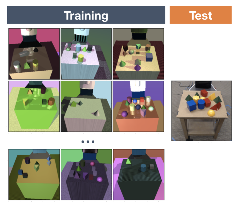
The randomization parameters can control appearances of the scene, including but not limited to the followings (see Fig. 2). A model trained on simulated and randomized images is able to transfer to real non-randomized images.

Position, shape, and color of objects,
Material texture,
Lighting condition,
Random noise added to images,
Position, orientation, and field of view of the camera in the simulator.

Fig. 2. Images captured in the training environment are randomized. (Image source: Tobin et al, 2017)

Physical dynamics in the simulator can also be randomized (Peng et al. 2018). Studies have showed that a recurrent policy can adapt to different physical dynamics including the partially observable reality. A set of physical dynamics features include but are not limited to:

Mass and dimensions of objects,
Mass and dimensions of robot bodies,
Damping, kp, friction of the joints,
Gains for the PID controller (P term),
Joint limit,
Action delay,
Observation noise.

With visual and dynamics DR, at OpenAI Robotics, we were able to learn a policy that works on real dexterous robot hand (OpenAI, 2018). Our manipulation task is to teach the robot hand to rotate an object continously to achieve 50 successive random target orientations. The sim2real gap in this task is very large, due to (a) a high number of simultaneous contacts between the robot and the object and (b) imperfect simulation of object collision and other motions. At first, the policy could barely survive for more than 5 seconds without dropping the object. But with the help of DR, the policy evolved to work surprisingly well in reality eventually.

Why does Domain Randomization Work?

Now you may ask, why does domain randomization work so well? The idea sounds really simple. Here are two non-exclusive explanations I found most convincing.

DR as Optimization

One idea (Vuong, et al, 2019) is to view learning randomization parameters in DR as a bilevel optimization. Assuming we have access to the real environment $e_\text{real}$ and the randomization config is sampled from a distribution parameterized by $\phi$, $\xi \sim P_\phi(\xi)$, we would like to learn a distribution on which a policy $\pi_\theta$ is trained on can achieve maximal performance in $e_\text{real}$:

$$ \begin{aligned} &\phi^* = \arg\min_{\phi} \mathcal{L}(\pi_{\theta^*(\phi)}; e_\text{real}) \\ \text{where } &\theta^*(\phi) = \arg\min_\theta \mathbb{E}_{\xi \sim P_\phi(\xi)}[\mathcal{L}(\pi_\theta; e_\xi)] \end{aligned} $$

where $\mathcal{L}(\pi; e)$ is the loss function of policy $\pi$ evaluated in the environment $e$.

Although randomization ranges are hand-picked in uniform DR, it often involves domain knowledge and a couple rounds of trial-and-error adjustment based on the transfer performance. Essentially this is a manual optimization process on tuning $\phi$ for the optimal $\mathcal{L}(\pi_{\theta^*(\phi)}; e_\text{real})$.

Guided domain randomization in the next section is largely inspired by this view, aiming to do bilevel optimization and learn the best parameter distribution automatically.

DR as Meta-Learning

In our learning dexterity project (OpenAI, 2018), we trained an LSTM policy to generalize across different environmental dynamics. We observed that once a robot achieved the first rotation, the time it needed for the following successes was much shorter. Also, a FF policy without memory was found not able to transfer to a physical robot. Both are evidence of the policy dynamically learning and adapting to a new environment.

In some ways, domain randomization composes a collection of different tasks. Memory in the recurrent network empowers the policy to achieve meta-learning across tasks and further work on a real-world setting.

Guided Domain Randomization

The vanilla DR assumes no access to the real data, and thus the randomization config is sampled as broadly and uniformly as possible in sim, hoping that the real environment could be covered under this broad distribution. It is reasonable to think of a more sophisticated strategy — replacing uniform sampling with guidance from task performance, real data, or simulator.

One motivation for guided DR is to save computation resources by avoiding training models in unrealistic environments. Another is to avoid infeasible solutions that might arise from overly wide randomization distributions and thus might hinder successful policy learning.

Optimization for Task Performance

Say we train a family of policies with different randomization parameters $\xi \sim P_\phi(\xi)$, where $P_\xi$ is the distribution for $\xi$ parameterized by $\phi$. Later we decide to try every one of them on the downstream task in the target domain (i.e. control a robot in reality or evaluate on a validation set) to collect feedback. This feedback tells us how good a configuration $\xi$ is and provides signals for optimizing $\phi$.

Inspired by NAS, AutoAugment (Cubuk, et al. 2018) frames the problem of learning best data augmentation operations (i.e. shearing, rotation, invert, etc.) for image classification as an RL problem. Note that AutoAugment is not proposed for sim2real transfer, but falls in the bucket of DR guided by task performance. Individual augmentation configuration is tested on the evaluation set and the performance improvement is used as a reward to train a PPO policy. This policy outputs different augmentation strategies for different datasets; for example, for CIFAR-10 AutoAugment mostly picks color-based transformations, while ImageNet prefers geometric based.

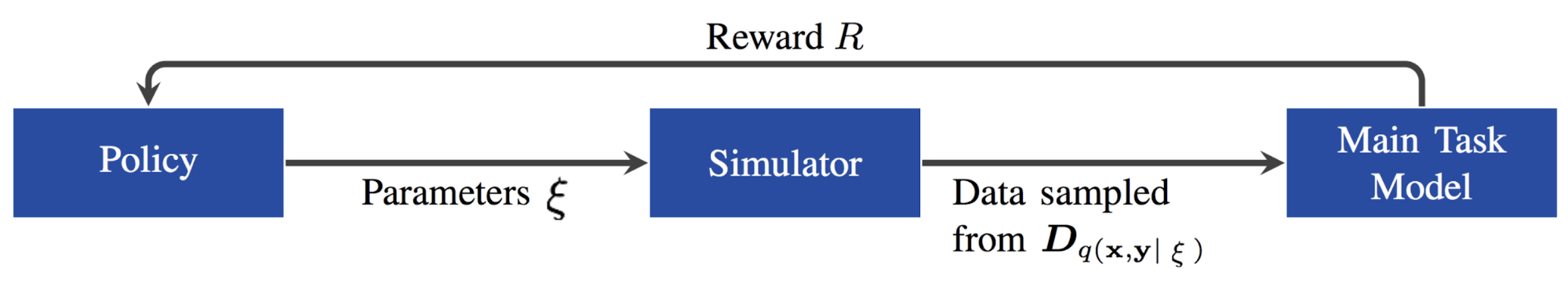
Ruiz (2019) considered the task feedback as reward in RL problem and proposed a RL-based method, named “learning to simulate”, for adjusting $\xi$. A policy is trained to predict $\xi$ using performance metrics on the validation data of the main task as rewards, which is modeled as a multivariate Gaussian. Overall the idea is similar to AutoAugment, applying NAS on data generation. According to their experiments, even if the main task model is not converged, it still can provide a reasonable signal to the data generation policy.

Fig. 3. An overview of the "learning to simulate" approach. (Image source: Ruiz (2019))

Evolutionary algorithm is another way to go, where the feedback is treated as fitness for guiding evolution (Yu et al, 2019). In this study, they used CMA-ES (covariance matrix adaptation evolution strategy) while fitness is the performance of a $\xi$-conditional policy in target environment. In the appendix, they compared CMA-ES with other ways of modeling the dynamics of $\xi$, including Bayesian optimization or a neural network. The main claim was those methods are not as stable or sample efficient as CMA-ES. Interestly, when modeling $P(\xi)$ as a neural network, LSTM is found to notably outperform FF.

Some believe that sim2real gap is a combination of appearance gap and content gap; i.e. most GAN-inspired DA models focus on appearance gap. Meta-Sim (Kar, et al. 2019) aims to close the content gap by generating task-specific synthetic datasets. Meta-Sim uses self-driving car training as an example and thus the scene could be very complicated. In this case, the synthetic scenes are parameterized by a hierarchy of objects with properties (i.e., location, color) as well as relationships between objects. The hierarchy is specified by a probabilistic scene grammar akin to structure domain randomization (SDR; Prakash et al., 2018) and it is assumed to be known beforehand. A model $G$ is trained to augment the distribution of scene properties $s$ by following:

Learn the prior first: pre-train $G$ to learn the identity function $G(s) = s$.
Minimize MMD loss between the real and sim data distributions. This involves backpropagation through non-differentiable renderer. The paper computes it numerically by perturbing the attributes of $G(s)$.
Minimize REINFORCE task loss when trained on synthetic data but evaluated on real data. Again, very similar to AutoAugment.

Unfortunately, this family of methods are not suitable for sim2real case. Either an RL policy or an EA model requires a large number of real samples. And it is really expensive to include real-time feedback collection on a physical robot into the training loop. Whether you want to trade less computation resource for real data collection would depend on your task.

Match Real Data Distribution

Using real data to guide domain randomization feels a lot like doing system identification or DA. The core idea behind DA is to improve the synthetic data to match the real data distribution. In the case of real-data-guided DR, we would like to learn the randomization parameters $\xi$ that bring the state distribution in simulator close to the state distribution in the real world.

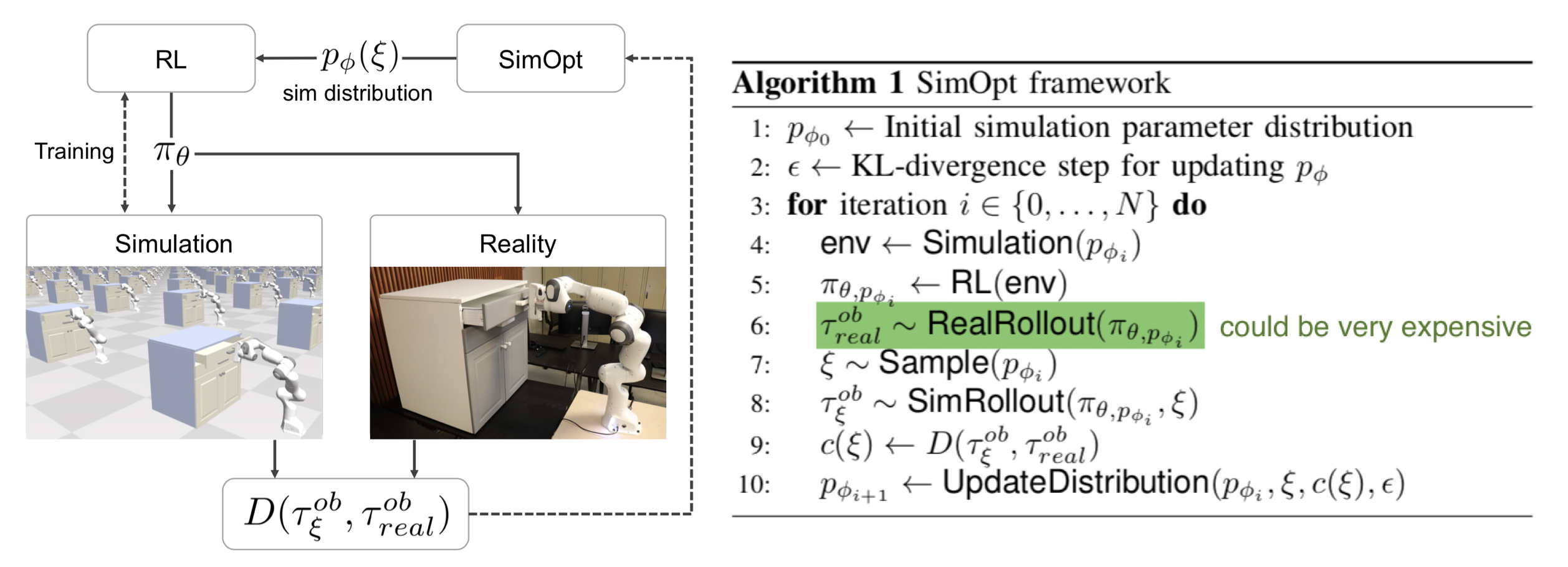
The SimOpt model (Chebotar et al, 2019) is trained under an initial randomization distribution $P_\phi(\xi)$ first, getting a policy $\pi_{\theta, P_\phi}$. Then this policy is deployed on both simulator and physical robot to collect trajectories $\tau_\xi$ and $\tau_\text{real}$ respectively. The optimization objective is to minimize the discrepancy between sim and real trajectories:

$$ \phi^* = \arg\min_{\phi}\mathbb{E}_{\xi \sim P_\phi(\xi)} [\mathbb{E}_{\pi_{\theta, P_\phi}} [D(\tau_\text{sim}, \tau_\text{real})]] $$

where $D(.)$ is a trajectory-based discrepancy measure. Like the “Learning to simulate” paper, SimOpt also has to solve the tricky problem of how to propagate gradient through non-differentiable simulator. It used a method called relative entropy policy search, see paper for more details.

Fig. 4. An overview of the SimOpt framework. (Image source: Chebotar et al, 2019)

RCAN (James et al., 2019), short for “Randomized-to-Canonical Adaptation Networks”, is a nice combination of DA and DR for end-to-end RL tasks. An image-conditional GAN (cGAN) is trained in sim to translate a domain-randomized image into a non-randomized version (aka “canonical version”). Later the same model is used to translate real images into corresponding simulated version so that the agent would consume consistent observation as what it has encountered in training. Still, the underlying assumption is that the distribution of domain-randomized sim images is broad enough to cover real-world samples.

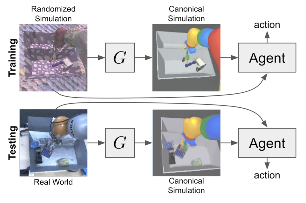
Fig. 5. RCAN is an image-conditional generator that can convert a domain-randomized or real image into its corresponding non-randomized simulator version. (Image source: James et al., 2019)

The RL model is trained end-to-end in a simulator to do vision-based robot arm grasping. Randomization is applied at each timestep, including the position of tray divider, objects to grasp, random textures, as well as the position, direction, and color of the lighting. The canonical version is the default simulator look. RCAN is trying to learn a generator

$G$: randomized image $\to$ {canonical image, segmentation, depth}

where segmentation masks and depth images are used as auxiliary tasks. RCAN had a better zero-shot transfer compared to uniform DR, although both were shown to be worse than the model trained on only real images. Conceptually, RCAN operates in a reverse direction of GraspGAN which translates synthetic images into real ones by domain adaptation.

Guided by Data in Simulator

Network-driven domain randomization (Zakharov et al., 2019), also known as DeceptionNet, is motivated by learning which randomizations are actually useful to bridge the domain gap for image classification tasks.

Randomization is applied through a set of deception modules with encoder-decoder architecture. The deception modules are specifically designed to transform images; such as change backgrounds, add distortion, change lightings, etc. The other recognition network handles the main task by running classification on transformed images.

The training involves two steps:

With the recognition network fixed, maximize the difference between the prediction and the labels by applying reversed gradients during backpropagation. So that the deception module can learn the most confusing tricks.
With the deception modules fixed, train the recognition network with input images altered.

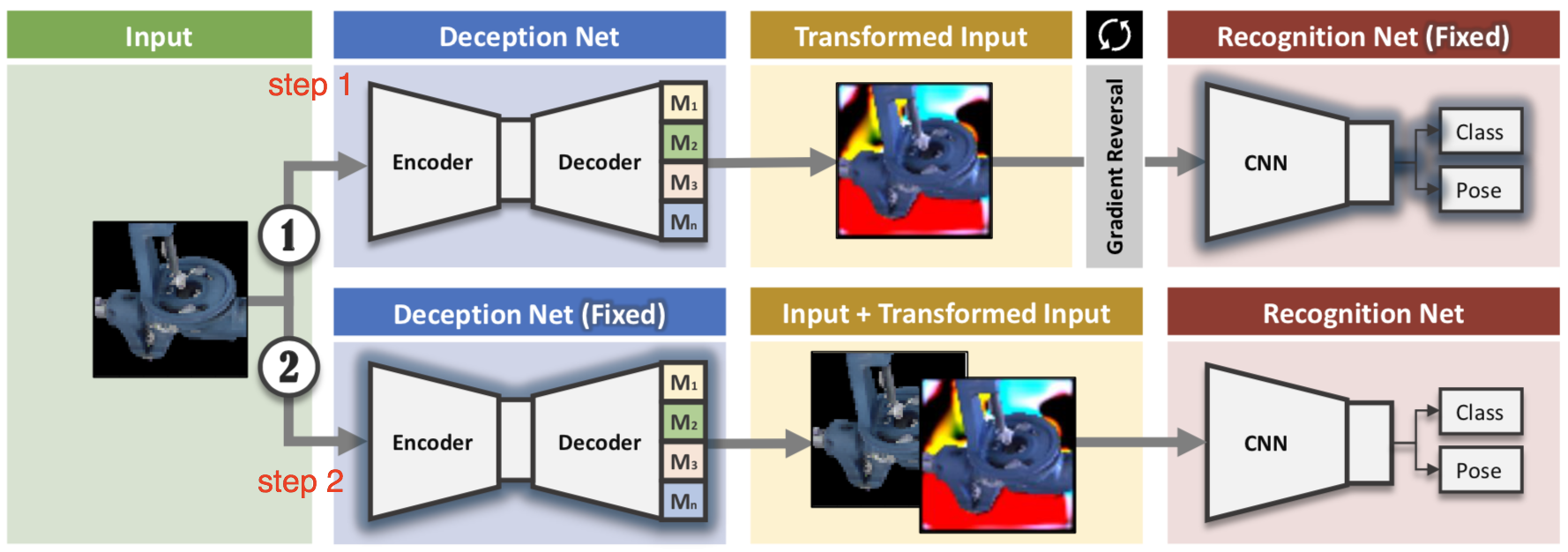
Fig. 6. How DeceptionNet works. (Image source: Zakharov et al., 2019)

The feedback for training deception modules is provided by the downstream classifier. But rather than trying to maximize the task performance like the section above, the randomization modules aim to create harder cases. One big disadvantage is you need to manually design different deception modules for different datasets or tasks, making it not easily scalable. Given the fact that it is zero-shot, the results are still worse than SOTA DA methods on MNIST and LineMOD.

Similarly, Active domain randomization (ADR; Mehta et al., 2019) also relies on sim data to create harder training samples. ADR searches for the most informative environment variations within the given randomization ranges, where the informativeness is measured as the discrepancies of policy rollouts in randomized and reference (original, non-randomized) environment instances. Sounds a bit like SimOpt? Well, noted that SimOpt measures the discrepancy between sim and real rollouts, while ADR measures between randomized and non-randomized sim, avoiding the expensive real data collection part.

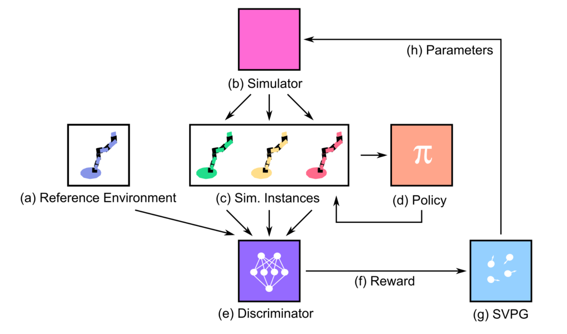
Fig. 7. How active domain randomization (ADR) works. (Image source: Mehta et al., 2019)

Precisely the training happens as follows:

Given a policy, run it on both reference and randomized envs and collect two sets of trajectories respectively.
Train a discriminator model to tell whether a rollout trajectory is randomized apart from reference run. The predicted $\log p$ (probability of being randomized) is used as reward. The more different randomized and reference rollouts, the easier the prediction, the higher the reward.
- The intuition is that if an environment is easy, the same policy agent can produce similar trajectories as in the reference one. Then the model should reward and explore hard environments by encouraging different behaviors.
The reward by discriminator is fed into Stein Variational Policy Gradient (SVPG) particles, outputting a diverse set of randomization configurations.

The idea of ADR is very appealing with two small concerns. The similarity between trajectories might not be a good way to measure the env difficulty when running a stochastic policy. The sim2real results look unfortunately not as exciting, but the paper pointed out the win being ADR explores a smaller range of randomization parameters.

Cited as:

@article{weng2019DR,
  title   = "Domain Randomization for Sim2Real Transfer",
  author  = "Weng, Lilian",
  journal = "lilianweng.github.io",
  year    = "2019",
  url     = "https://lilianweng.github.io/posts/2019-05-05-domain-randomization/"
}

Overall, after reading this post, I hope you like domain randomization as much as I do :).

References

[1] Josh Tobin, et al. “Domain randomization for transferring deep neural networks from simulation to the real world.” IROS, 2017.
[2] Fereshteh Sadeghi and Sergey Levine. “CAD2RL: Real single-image flight without a single real image.” arXiv:1611.04201 (2016).
[3] Xue Bin Peng, et al. “Sim-to-real transfer of robotic control with dynamics randomization.” ICRA, 2018.
[4] Nataniel Ruiz, et al. “Learning to Simulate.” ICLR 2019
[5] OpenAI. “Learning Dexterous In-Hand Manipulation.” arXiv:1808.00177 (2018).
[6] OpenAI Blog. “Learning dexterity” July 30, 2018.
[7] Quan Vuong, et al. “How to pick the domain randomization parameters for sim-to-real transfer of reinforcement learning policies?.” arXiv:1903.11774 (2019).
[8] Ekin D. Cubuk, et al. “AutoAugment: Learning augmentation policies from data.” arXiv:1805.09501 (2018).
[9] Wenhao Yu et al. “Policy Transfer with Strategy Optimization.” ICLR 2019
[10] Yevgen Chebotar et al. “Closing the Sim-to-Real Loop: Adapting Simulation Randomization with Real World Experience.” Arxiv: 1810.05687 (2019).
[11] Stephen James et al. “Sim-to-real via sim-to-sim: Data-efficient robotic grasping via randomized-to-canonical adaptation networks” CVPR 2019.
[12] Bhairav Mehta et al. “Active Domain Randomization” arXiv:1904.04762
[13] Sergey Zakharov,et al. “DeceptionNet: Network-Driven Domain Randomization.” arXiv:1904.02750 (2019).
[14] Amlan Kar, et al. “Meta-Sim: Learning to Generate Synthetic Datasets.” arXiv:1904.11621 (2019).
[15] Aayush Prakash, et al. “Structured Domain Randomization: Bridging the Reality Gap by Context-Aware Synthetic Data.” arXiv:1810.10093 (2018).